Plotting spectra

Plot the spectra of a hyperSpec object, i.e. intensity over wavelength. Instead of the intensity values of the spectra matrix summary values calculated from these may be used.

Usually, the stacked argument of plotspc() will do fine, but if you need fine control over the stacking, you may calculate the y offsets yourself.

plotspc(
  object,
  wl.range = TRUE,
  wl.index = FALSE,
  wl.reverse = FALSE,
  spc.nmax = hy.getOption("plot.spc.nmax"),
  func = NULL,
  func.args = list(),
  stacked = NULL,
  stacked.args = list(),
  add = FALSE,
  bty = "l",
  plot.args = list(),
  col = "black",
  lines.args = list(),
  xoffset = 0,
  yoffset = 0,
  nxticks = 10,
  axis.args = list(),
  break.args = list(),
  title.args = list(),
  fill = NULL,
  fill.col = NULL,
  border = NA,
  polygon.args = list(),
  zeroline = list(lty = 2, col = col),
  debuglevel = hy.getOption("debuglevel")
)

stacked.offsets(
  x,
  stacked = TRUE,
  min.zero = FALSE,
  add.factor = 0.05,
  add.sum = 0,
  .spc = NULL,
  debuglevel = hy.getOption("debuglevel")
)

Arguments

object	the hyperSpec object
wl.range	the wavelength range to be plotted. Either a numeric vector or a list of vectors with different wavelength ranges to be plotted separately. The values can be either wavelengths or wavelength indices (according to wl.index).
wl.index	if TRUE, wl.range is considered to give column indices into the spectra matrix. Defaults to specifying wavelength values rather than indices.
wl.reverse	if TRUE, the wavelength axis is plotted backwards.
spc.nmax	maximal number of spectra to be plotted (to avoid accidentally plotting of large numbers of spectra).
func	a function to apply to each wavelength in order to calculate summary spectra such as mean, min, max, etc.
func.args	list with furter arguments for func
stacked	if not NULL, a "stacked" plot is produced, see the example. stacked may be TRUE to stack single spectra. A numeric or factor is interpreted as giving the grouping, character is interpreted as the name of the extra data column that holds the groups.
stacked.args	a list with further arguments to stacked.offsets().
add	if TRUE, the output is added to the existing plot
bty	see graphics::par()
plot.args	list with further arguments to graphics::plot()
col	see graphics::par(). col might be a vector giving individual colors for the spectra.
lines.args	list with further arguments to graphics::lines(). lines.args$type defaults to "l".
xoffset	vector with abscissa offsets for each of the wl.ranges. If it has one element less than there are wl.ranges, 0 is padded at the beginning. The values are interpreted as the distance along the wavelength axis that the following parts of the spectra are shifted towards the origin. E.g. if wl.range = list (600 ~ 1800, 2800 ~ 3200), xoffset = 750 would result in a reasonable plot. See also the examples.
yoffset	ordinate offset values for the spectra. May be offsets to stack the spectra (stacked.offsets()). Either one for all spectra, one per spectrum or one per group in stacked.
nxticks	hint how many tick marks the abscissa should have.
axis.args	list with further arguments for graphics::axis(). axis.args$x should contain arguments for plotting the abscissa, axis.args$y those for the ordinate (again as lists).
break.args	list with arguments for plotrix::axis.break().
title.args	list with further arguments to graphics::title(). title.args may contain two lists, $x, and $y to set parameters individually for each axis.
fill	if not NULL, the area between the specified spectra is filled with color col. The grouping can be given as factor or numeric, or as a character with the name of the extra data column to use. If a group contains more than 2 spectra, the first and the last are used. If TRUE spectra n and nrow (spc) - n build a group.
fill.col	character vector with fill color. Defaults to brightened colors from col.
border	character vector with border color. You will need to set the line color col to NA in order see the effect.
polygon.args	list with further arguments to graphics::polygon() which draws the filled areas.
zeroline	NA or a list with arguments graphics::abline(), used to plot line (s) marking I = 0. NA suppresses plotting of the line. The line is by default turned off if yoffset is not 0.
debuglevel	if > 0, additional debug output is produced, see options() for details
x	a hyperSpec object
min.zero	if TRUE, the lesser of zero and the minimum intensity of the spectrum is used as minimum.
add.factor, add.sum	proportion and absolute amount of space that should be added.
.spc	for internal use. If given, the ranges are evaluated on .spc. However, this may change in future.

Value

plotspc invisibly returns a list with

x

the abscissa coordinates of the plotted spectral data points

y

a matrix the ordinate coordinates of the plotted spectral data points

wavelengths

the wavelengths of the plotted spectral data points

This can be used together with spc.identify(). a list containing

offsets

numeric with the yoffset for each group in stacked

groups

numeric with the group number for each spectrum

levels

if stacked is a factor, the levels of the groups

Details

This is hyperSpec's main plotting function for spectra plots.

New plots are created by graphics::plot(), but the abscissa and ordinate are drawn separately by graphics::axis(). Also, graphics::title() is called explicitly to set up titles and axis labels. This allows fine-grained customization of the plots.

If package plotrix is available, its function plotrix::axis.break() is used to produce break marks for cut wavelength axes.

Empty levels of the stacking factor are dropped (as no stacking offset can be calculated in that case.)

See also

graphics::plot(), graphics::axis(), graphics::title(), graphics::lines(), graphics::polygon(), graphics::par() for the description of the respective arguments.

plotrix::axis.break() for cut marks

See plot() for some predefined spectra plots such as mean spectrum +/- one standard deviation and the like.

graphics::identify() and graphics::locator() about interaction with plots.

plotspc()

Author

C. Beleites

C. Beleites

Examples

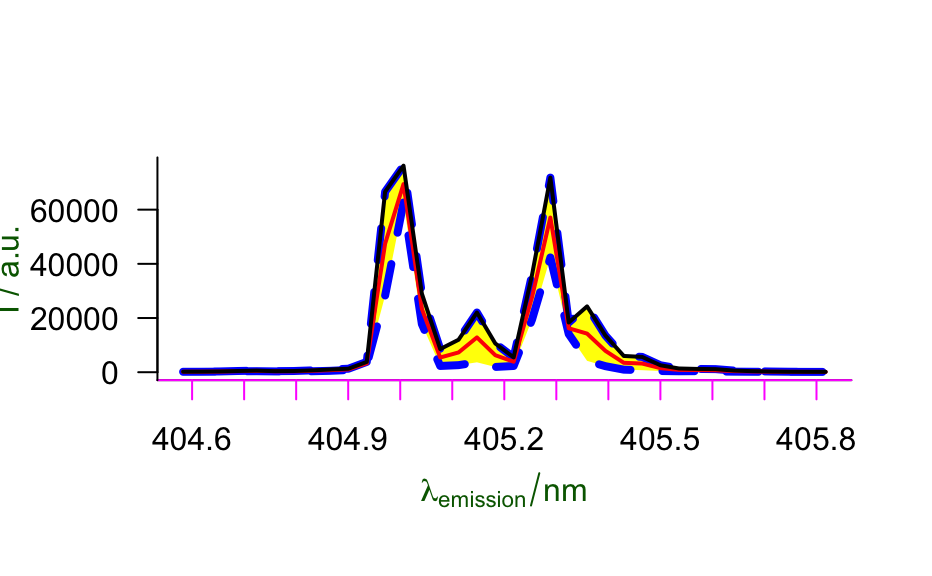
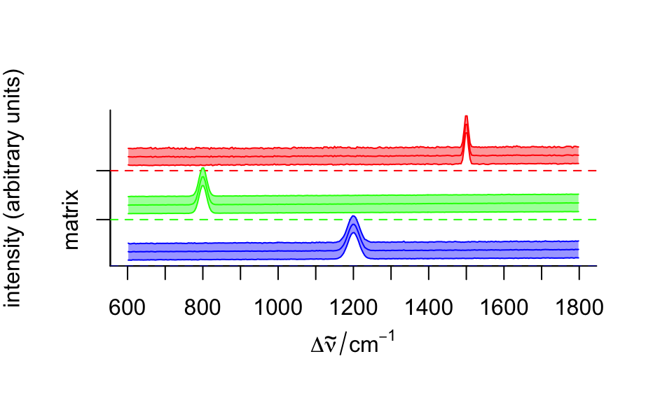
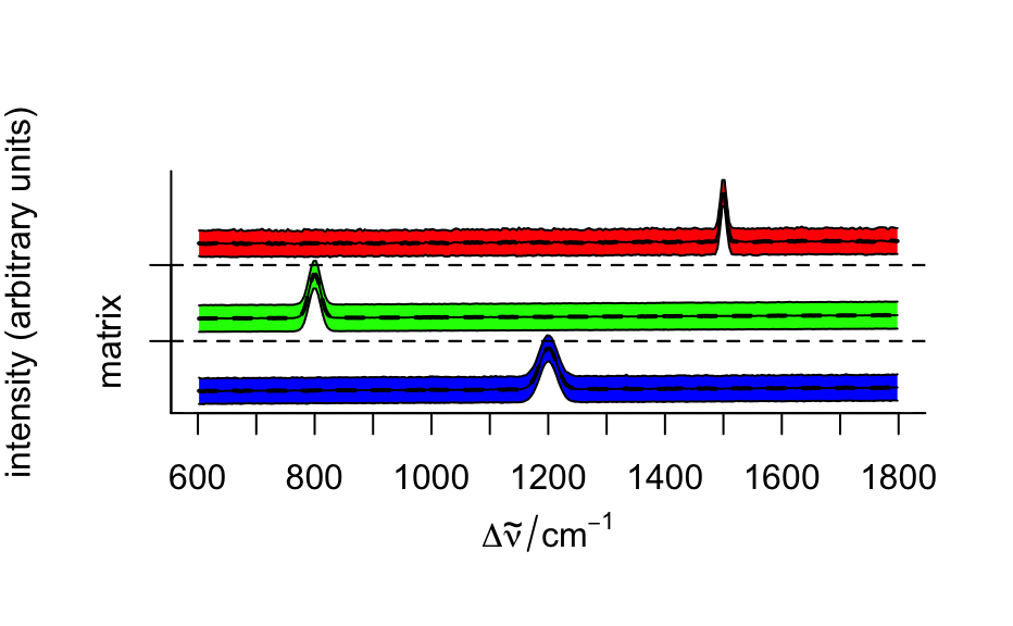
plotspc(flu)

## artificial example to show wavelength axis cutting
plotspc(faux_cell[sample(nrow(faux_cell), 50)],
  wl.range = list(600 ~ 650, 1000 ~ 1100, 1600 ~ 1700),
  xoffset = c(0, 300, 450)
)

plotspc(faux_cell[sample(nrow(faux_cell), 50)],
  wl.range = list(600 ~ 650, 1000 ~ 1100, 1600 ~ 1700),
  xoffset = c(300, 450)
)

## some journals publish Raman spectra backwards
plotspc(faux_cell[sample(nrow(faux_cell), 50)], wl.reverse = TRUE)

plotspc(laser[(0:4) * 20 + 1, , ], stacked = TRUE)

plotspc(laser,
  func = mean_pm_sd,
  col = c(NA, "red", "black"), lines.args = list(lwd = 2),
  fill = c(1, NA, 1),
  fill.col = "yellow", border = "blue",
  polygon.args = list(lty = 2, lwd = 4),
  title.args = list(
    xlab = expression(lambda[emission] / nm),
    y = list(line = 3.4),
    col.lab = "darkgreen"
  ),
  axis.args = list(x = list(col = "magenta"), y = list(las = 1))
)

mean.pm.sd <- aggregate(faux_cell, faux_cell$region, mean_pm_sd)
plot(mean.pm.sd, col = palette_matlab(3), fill = ".aggregate", stacked = ".aggregate")

mean.pm.sd <- aggregate(faux_cell, faux_cell$region, mean_pm_sd)

offset <- stacked.offsets(mean.pm.sd, ".aggregate")
plot(mean.pm.sd,
  fill.col = palette_matlab(3), fill = ".aggregate",
  stacked = ".aggregate"
)

plot(aggregate(faux_cell, faux_cell$region, mean),
  yoffset = offset$offsets,
  lines.args = list(lty = 2, lwd = 2), add = TRUE
)

barb <- do.call(collapse, barbiturates[1:3])
plot(barb,
  lines.args = list(type = "h"), stacked = TRUE,
  stacked.args = list(add.factor = .2)
)