Introduction to Package “hyperSpec”

The Main Manual of Package “hyperSpec”

Claudia Beleites^1,2,3,4,5, Vilmantas Gegzna, Bryan A. Hanson

DIA Raman Spectroscopy Group, University of Trieste/Italy (2005–2008)
Spectroscopy $\cdot$ Imaging, IPHT, Jena/Germany (2008–2017)
ÖPV, JKI, Berlin/Germany (2017–2019)
Arbeitskreis Lebensmittelmikrobiologie und Biotechnologie, Hamburg University, Hamburg/Germany (2019 – 2020)
Chemometric Consulting and Chemometrix GmbH, Wölfersheim/Germany (since 2016)

chemometrie@beleites.de

2021-07-14

Source: ../vignettes/hyperSpec.Rmd

hyperSpec.Rmd

Note:

Package hyperSpec and it’s friends provide a number of vignettes to help you get started.

You can access the vignettes via these links:
Alternatively, if you are offline or prefer accessing the vignettes with R, simply type browseVignettes(“hyperSpec”) to get a clickable list in a browser window.
Vignettes in other packages:
- Example Workflow for 2D Raman Spectra (chondro dataset)
- Plotting hyperSpec objects with ggplot2
- Using dplyr functions with hyperSpec objects

1 Things to Know About hyperSpec

Package hyperSpec is a R package that allows convenient handling of hyperspectral data sets, i.e., data sets combining spectra with further data on a per-spectrum basis. The spectra can be anything that is recorded over a common discretized axis. This vignette gives an introduction on basic working techniques using the R package package hyperSpec. This is done mostly from a spectroscopic point of view: rather than going through the functions provided by package hyperSpec, it is organized by spectroscopic tasks.

1.1 Terms & Notations Used Here

Throughout the documentation of the package, the following terms are used:

wavelength: spectral abscissa frequency, typical units are wavenumbers, chemical shift, Raman shift, $\frac{m}{z}$, etc.
intensity: spectral ordinate transmission, absorbance, $\frac{e^{-}}{s}$, intensity, etc.
extra data: further information/data belonging to each spectrum such as spatial information (spectral images, maps, or profiles), temporal information (kinetics, time series), concentrations (calibration series), class membership information, etc. Class hyperSpec object may contain arbitrary numbers of extra data columns.

In R, slots of an S4 class are accessed by the @ operator. In this vignette, the notation @xxx will thus mean “slot xxx of an object”. Likewise, named elements of a list and columns of a data.frame are accessed by the $ operator, and $xxx will be used for “column xxx”, and as an abbreviation for “column xxx of the data.frame in slot data of the object” (the structure of hyperSpec objects is discussed in section 1.2).

1.2 The Structure of hyperSpec Objects

hyperSpec objects are defined using an S4 class. It contains the following slots:

@wavelength containing a numeric vector with the wavelength axis of the spectra.
@data a data.frame with the spectra and all further information belonging to the spectra.
@label a list with appropriate labels (particularly for axis annotations).

Most of the data is stored in @data. This data.frame has one special column, $spc. This is the column that actually contains the spectra. The spectra are stored in a matrix inside this column, as illustrated in Figure 1.1. Even if there are no spectra, $spc must still be present. It is then a matrix with zero columns.

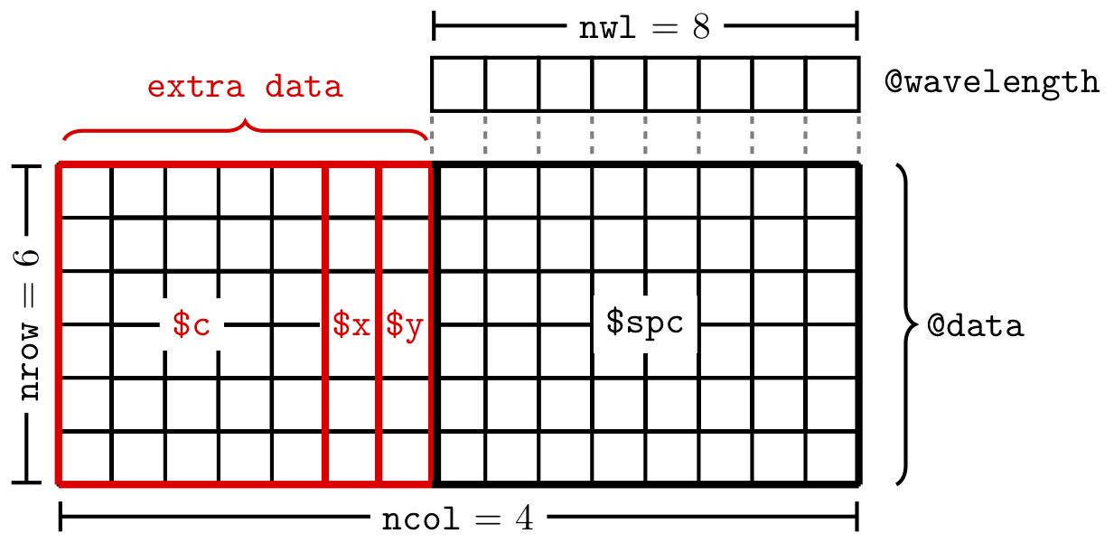
Figure 1.1: The structure of the data in a hyperSpec object. In this example the ‘extra data’ are the x, y and c columns in @data.

Slot @label contains an element for each of the columns in @data plus one holding the label for the wavelength axis, .wavelength. They are accessed by their names which must be the same for columns of @data and the list elements. The elements of the list may be anything suitable for axis annotations, i.e., they should be either character strings or expressions for “pretty” axis annotations (see, e.g., Figure 5.7). To get familiar with expressions for axis annotation, see ?plotmath and demo(plotmath).

1.3 Data Sets

Package hyperSpec comes with several data sets:

`flu`	A set of fluorescence spectra of a calibration series.
`laser`	A time series of an unstable laser emission.
`paracetamol`	A Raman spectrum of paracetamol (acetaminophen) ranging from 100 to 3200 cm^-1 with overlapping wavelength ranges.
`faux_cell`	A synthetic data set similar to `chondro`.
`barbiturates`	GC-MS spectra with differing wavelength axes as a list of 5 hyperSpec objects.

In this vignette, the data sets are used to illustrate appropriate procedures for different tasks and different spectra. In addition, laser and flu are accompanied by their own vignettes showing sample work flows for the respective data type.

This document describes how to accomplish typical tasks in the analysis of spectra. It does not give a complete reference on particular functions. It is therefore recommended to look up the methods in the R help system using ?command.

1.4 Options

The global behaviour of package hyperSpec can be configured via options. The values of the options are retrieved with hy.getOptions() and hy.getOption(), and changed with hy.setOptions(). Table 9.1 gives an overview of the options. You should not worry about these at the start of your exploration of hyperSpec.

2 Obtaining Basic Information about hyperSpec Objects

Any of print(), show() or summary() provides an overview of the object (the output of each is identical):

faux_cell
#> hyperSpec object
#>    875 spectra
#>    4 data columns
#>    300 data points / spectrum

The data set faux_cell consists of 875 spectra with 300 data points each, and 4 data columns: two for the spatial information, one giving the cell region of each pixel plus $spc. These details can be directly obtained by

nrow(faux_cell)
#> [1] 875

nwl(faux_cell)
#> [1] 300

ncol(faux_cell)
#> [1] 4

dim(faux_cell)
#> nrow ncol  nwl 
#>  875    4  300

The names of the columns in @data are accessed by colnames().

colnames(faux_cell)
#> [1] "x"      "y"      "region" "spc"

Likewise, rownames() returns the names assigned to the spectra, and dimnames() yields a list of these three vectors (including also the column names of $spc). The column names of the spectra matrix contain the wavelengths as a character vector, while wl() (see section 3.6.4) returns the numeric vector of wavelengths.

3 Accessing & Manipulating hyperSpec Objects

While the parts of the hyperSpec object can be accessed directly, it is good practice to use the functions provided by the package to handle the objects rather than accessing the slots directly. This also ensures that proper (i.e. valid) objects are returned. In some cases, however, direct access to the slots can considerably speed up calculations (see the appendicies).

The main functions to retrieve the data of a hyperSpec object are [] and [[]]. The difference between these functions is that [] returns a hyperSpec object, whereas [[]] returns a data.frame containing x$spc, the spectral data. To modify a hyperSpec object, the corresponding functions are [<- and [[<-. The first form is used to modify the entire hyperSpec object and the second form modifies the spectral data in x$spc.

hyperSpec objects are triple indexed:

x[i, j, l, wl.index = TRUE/FALSE]
x[[i, j, l, wl.ndex = TRUE/FALSE]]
i refers to rows of the @data slot. i can be integer indices or a logical vector.
j refers to columns of the @data slot. j can be integer indices, a logical vector or the name of a column. However, there is no guaranteed order to colnames(x) so using integer indices and logical vectors is unwise.
l refers to wavelengths. Note the argument wl.index which determines how l is interpreted.
If there is only one index given, e.g. x[1:3], it refers to the row index i. Likewise if there are only two indices given they refer to i and j.
See 3.5.1 and 3.4 for even more ways to specify the indices.

3.1 Summary of Extraction Functions for hyperSpec Objects (getters)

Table 3.1 shows the main functions that can be used with class hyperSpec to access the object (“getters”).

**Table 3.1:** Getter functions for the slots of `hyperSpec` objects
`x[]`	Returns the entire `hyperSpec` object unchanged.
`x[i, , ]`	Returns the `hyperSpec` object with selected rows; equivalent to `x[i]`.
`x[, j, ]`	Returns the `hyperSpec` object with empty `x$spc` slot. If you want the column `j`, `x[["name"]]` returns a `data.frame` containing `j` or `x$name` returns it as a vector.
`x[, , l, wl.index = TRUE/FALSE]`	Returns the `hyperSpec` object with selected wavelengths.
`x[[]]`	Returns the spectra matrix (`x$spc`).
`x[[i, , ]]`	Returns the spectra matrix (`x$spc`) with selected rows.
`x[[, j, ]]`	Returns a `data.frame` with the selected columns. Safest to give `j` as a character string.
`x[[, , l, wl.index = TRUE/FALSE]]`	Returns the spectra matrix (`x$spc`) with selected wavelengths.
`x$name`	Returns the column `name` as a vector.
`x$.`	Returns the complete `data.frame` `x@data`, with the spectra in column `$spc`.
`x$..`	Returns all the extra data (`x@data` without `x$spc`).
`wl()`	Returns the wavelengths.
`labels()`	Returns the labels.

One can see that there are several ways to get the spectral data: x$spc, x[[]], x$... The first two forms return a matrix, while the last returns a data.frame.

3.2 Summary of Replacement Functions for hyperSpec Objects (setters)

Table 3.2 shows the main functions that can be used with class hyperSpec to modify the object (“setters”).

**Table 3.2:** Setter functions for the slots of `hyperSpec` objects
`x[i, ,] <-`	Replaces the specified rows of the `@data` slot, including `x$spc` and any extra data columns. Other approaches are probably easier.
`x[, j,] <-`	Replaces the specified columns. Safest to give `j` as a character string.
`x[i, j] <-`	Replaces the specified column limited to the specified rows. Safest to give `j` as a character string.`x[, , l, wl.index = TRUE/FALSE] <-` Replaces the specified wavelengths.
`x[[i, ,]] <-`	Replaces the specified row of `x$spc`
`x[[, j,]] <-`	As `[[]]` refers to just the spectral data in `x$spc`, this operation is not valid. See below.
`x[[, , l, wl.index = TRUE/FALSE]] <-`	Replaces the intensity values in `x$spc` for the specified wavelengths.
`x[[i, , l, wl.index = TRUE/FALSE]] <-`	Replaces the intensity values in `x$spc` for the specified wavelengths limited to the specified rows.
`x$.. <-`	Sets the extra data (`x@data` without touching `x$spc`). The column names must match exactly in this case.
`wl<-`	Sets the wavelength vector.
`labels<-`	Sets the labels.

For more details on []<-, [[]]<-, and $<-, see 3.5.1 and 3.4.

3.3 Selecting and Deleting Spectra

The extraction function [] takes the spectra (rows) as the first argument (For detailed help: see ?"["). It may be a vector giving the indices of the spectra to extract (select), a vector with negative indices indicating, which spectra should be deleted, or a vector of logical values.

data(palette_colorblind) # load colorblind-friendly palette
plot(flu, col = palette_colorblind[4])
plot(flu[1:3], add = TRUE)

Figure 3.1: An example with [] operator and positive indices.

plot(flu, col = palette_colorblind[4])
plot(flu[-3], add = TRUE)

Figure 3.2: An example with [] operator and negative indices.

plot(flu, col = palette_colorblind[4])
plot(flu[flu$c > 0.2], add = TRUE)

Figure 3.3: An example with [] operator and logical indices.

3.3.1 Random Samples

A random subset of spectra can be conveniently selected by sample():

sample(faux_cell, 3)
#> hyperSpec object
#>    3 spectra
#>    4 data columns
#>    300 data points / spectrum

If indices into the selected spectra are needed instead, use isample():

isample(faux_cell, 3)
#> [1] 183 797 279

3.3.2 Sequences

Sequences of every n^th spectrum or the like can be retrieved with seq():

seq(faux_cell, length.out = 3, index = TRUE)
#> [1]   1 438 875
seq(faux_cell, by = 100)
#> hyperSpec object
#>    9 spectra
#>    4 data columns
#>    300 data points / spectrum

Here, indices may be requested using index = TRUE.

3.4 Selecting Extra Data Columns

The second argument of the extraction functions [] and [[]] specifies the extra data columns. They can be given like any column specification for a data.frame, i.e., numeric, logical, or by a vector of the column names. However, since there is intrinsic order the column names of a hyperSpec object, using the column names is safest:

colnames(faux_cell)
#> [1] "x"      "y"      "region" "spc"

faux_cell[[1:3, 1]]
#>        x
#> 1 -11.55
#> 2 -10.55
#> 3  -9.55

faux_cell[[1:3, -5]]
#>        x     y region spc.602 spc.606 spc.610 spc.614 spc.618 spc.622 spc.626 spc.630 spc.634
#> 1 -11.55 -4.77 matrix     132     132     150     128     143     113     121     125     121
#> 2 -10.55 -4.77 matrix      72      73      99      84      54      74      68      79      73
#> 3  -9.55 -4.77 matrix     120     132     142     118     125     123     111     146     122
#>   spc.638 spc.642 spc.646 spc.650 spc.654 spc.658 spc.662 spc.666 spc.670 spc.674 spc.678 spc.682
#> 1     123     135     139     151     143     133     113     124     104     127     127     131
#> 2      98      83      74      73      69      90      84      80      69      61      65      76
#> 3     123     142     137     141     114     127     120     137     115     127     137     142
#>   spc.686 spc.690 spc.694 spc.698 spc.702 spc.706 spc.710 spc.714 spc.718 spc.722 spc.726 spc.730
#> 1     145     134     127     136     121     131     132     131     141     139     109     124
#> 2      80      93      76      80      79      93      81      72      74      76      90      78
#> 3     128     137     118     115     116     126     116     125     111     125     106     123
#>   spc.734 spc.738 spc.742 spc.746 spc.750 spc.754 spc.758 spc.762 spc.766 spc.770 spc.774 spc.778
#> 1     136     124     111     127     128     152     133     122     166     132     146     136
#> 2      78      94      86      72      77      76      79      91      69      63      84     109
#> 3     128     119     111     142     139     123     111     138     119     109     126     111
#>   spc.782 spc.786 spc.790 spc.794 spc.798 spc.802 spc.806 spc.810 spc.814 spc.818 spc.822 spc.826
#> 1     159     232     267     288     324     312     263     267     216     185     130     150
#> 2     129     160     193     237     260     272     238     203     154     115     104      93
#> 3     172     216     267     282     313     324     280     232     186     182     127     127
#>   spc.830 spc.834 spc.838 spc.842 spc.846 spc.850 spc.854 spc.858 spc.862 spc.866 spc.870 spc.874
#> 1     136     156     123     123     131     131     134     128     133     151     143     124
#> 2      98      71      77      66      92      64      84      80      75      79      81      77
#> 3     117     135     123     119     121     125     134     130     125     136     125     135
#>   spc.878 spc.882 spc.886 spc.890 spc.894 spc.898 spc.902 spc.906 spc.910 spc.914 spc.918 spc.922
#> 1     132     120     123     117     111     128     117     145     147     116     121     137
#> 2      85      82      85      74      81      76      66      77      74      81      87      85
#> 3     117     144     126     143     148     124     138     131     126     138     110     132
#>   spc.926 spc.930 spc.934 spc.938 spc.942 spc.946 spc.950 spc.954 spc.958 spc.962 spc.966 spc.970
#> 1     147     124     137     139     143     128     123     113     120     139     162     108
#> 2      72      91      94      69      75      81      72      84      82      80      70      80
#> 3     135     140     131     123     144     126     118     135     138     144     142     116
#>   spc.974 spc.978 spc.982 spc.986 spc.990 spc.994 spc.998 spc.1002 spc.1006 spc.1010 spc.1014
#> 1     141     138     132     145     122     118     105      116      132      122      137
#> 2      86      84      78      80      97      83      66       67       78       90       77
#> 3     146     139     135     134     131     143     135      128      131      139      128
#>   spc.1018 spc.1022 spc.1026 spc.1030 spc.1034 spc.1038 spc.1042 spc.1046 spc.1050 spc.1054
#> 1      133      105      114      127      129      142      139      122      114      122
#> 2       89       74       76       82       79       96       83       72       69       86
#> 3      119      126      136      136      138      113      126      150      115      133
#>   spc.1058 spc.1062 spc.1066 spc.1070 spc.1074 spc.1078 spc.1082 spc.1086 spc.1090 spc.1094
#> 1      130      136      143      116      147      132      138      137      108      130
#> 2       84       83       95       66       95       96       87       90       80       85
#> 3      126      130      135      133      124      141      135      131      128      141
#>   spc.1098 spc.1102 spc.1106 spc.1110 spc.1114 spc.1118 spc.1122 spc.1126 spc.1130 spc.1134
#> 1      154      134      125      155      123      111      132      146      146      122
#> 2       77       88       74       86       76       70       85       71       71       94
#> 3      136      124      136      132      116      148      144      145      147      124
#>   spc.1138 spc.1142 spc.1146 spc.1150 spc.1154 spc.1158 spc.1162 spc.1166 spc.1170 spc.1174
#> 1      130      123      122      131      150      144      129      132      133      130
#> 2       96       72       75       86       85       81       87       75       72       82
#> 3      147      137      144      126      124      146      121      155      139      150
#>   spc.1178 spc.1182 spc.1186 spc.1190 spc.1194 spc.1198 spc.1202 spc.1206 spc.1210 spc.1214
#> 1      125      118      113      141      131      117      129      136      120      124
#> 2       81       87       82       84       77       80       60       87       81       89
#> 3      103      120      126      135      147      138      124      127      128      124
#>   spc.1218 spc.1222 spc.1226 spc.1230 spc.1234 spc.1238 spc.1242 spc.1246 spc.1250 spc.1254
#> 1      152      117      126      126      151      132      134      138      127      117
#> 2       74       80       71       88       77       95       75       78       76       79
#> 3      132      135      151      137      136      132      135      138      136      109
#>   spc.1258 spc.1262 spc.1266 spc.1270 spc.1274 spc.1278 spc.1282 spc.1286 spc.1290 spc.1294
#> 1      134      131      122      128      128      153      131      116      143      127
#> 2       81       85       92       83       88       79       88       90       81       87
#> 3      158      143      135      122      129      127      128      135      134      123
#>   spc.1298 spc.1302 spc.1306 spc.1310 spc.1314 spc.1318 spc.1322 spc.1326 spc.1330 spc.1334
#> 1      120      125      111      132      144      129      124      128      124      121
#> 2       73       78       91       79       95       96       90       69       87       82
#> 3      140      140      128      134      139      116      123      145      128      134
#>   spc.1338 spc.1342 spc.1346 spc.1350 spc.1354 spc.1358 spc.1362 spc.1366 spc.1370 spc.1374
#> 1      123      134      140      136      141      131      149      117      131      134
#> 2       90      101       79       69       63       83       84       73       85       78
#> 3      125      146      149      145      145      129      132      116      126      123
#>   spc.1378 spc.1382 spc.1386 spc.1390 spc.1394 spc.1398 spc.1402 spc.1406 spc.1410 spc.1414
#> 1      115      154      127      123      124      120      170      130      138      139
#> 2       77       82       92       92       87       79       77       80       89       75
#> 3      133      136      151      133      165      148      150      111      133      133
#>   spc.1418 spc.1422 spc.1426 spc.1430 spc.1434 spc.1438 spc.1442 spc.1446 spc.1450 spc.1454
#> 1      128      125      134      139      157      130      146      131      128      137
#> 2       89       78      100       83       80       91       84       98       82       95
#> 3      125      146      142      143      101      149      130      139      135      143
#>   spc.1458 spc.1462 spc.1466 spc.1470 spc.1474 spc.1478 spc.1482 spc.1486 spc.1490 spc.1494
#> 1      142      130      143      121      123      138      148      131      132      125
#> 2       72       95       85       93       84      101       94       95       90       73
#> 3      133      149      144      132      147      150      145      130      122      116
#>   spc.1498 spc.1502 spc.1506 spc.1510 spc.1514 spc.1518 spc.1522 spc.1526 spc.1530 spc.1534
#> 1      126      134      112      117      120      145      148      134      131      121
#> 2       84       78       92       70       80       82       78       87       87      105
#> 3      143      122      134      132      149      121      158      143      123      143
#>   spc.1538 spc.1542 spc.1546 spc.1550 spc.1554 spc.1558 spc.1562 spc.1566 spc.1570 spc.1574
#> 1      143      116      134      123      132      135      117      130      129      118
#> 2       84       85       76       86       90       87       86       86       95       69
#> 3      160      127      143      149      140      129      145      137      149      138
#>   spc.1578 spc.1582 spc.1586 spc.1590 spc.1594 spc.1598 spc.1602 spc.1606 spc.1610 spc.1614
#> 1      122      139      109      115      154      118      124      131      123      148
#> 2       94       97       92       79       90       72       82       81       79       90
#> 3      134      168      154      134      134      153      132      148      129      152
#>   spc.1618 spc.1622 spc.1626 spc.1630 spc.1634 spc.1638 spc.1642 spc.1646 spc.1650 spc.1654
#> 1      134      132      132      115      125      119      130      129      128      118
#> 2       90       79       94       84      105       71       74       88       83       74
#> 3      149      147      148      138      166      152      122      144      124      150
#>   spc.1658 spc.1662 spc.1666 spc.1670 spc.1674 spc.1678 spc.1682 spc.1686 spc.1690 spc.1694
#> 1      128      143      113      143      128      126      121      126      134      126
#> 2       81       82      104       85       76       98       79       85      108       86
#> 3      128      140      144      127      124      131      143      142      135      134
#>   spc.1698 spc.1702 spc.1706 spc.1710 spc.1714 spc.1718 spc.1722 spc.1726 spc.1730 spc.1734
#> 1      151      125      159      130      130      139      127      129      122      138
#> 2       65       75       93       95       94       77       73       82       83       85
#> 3      124      147      133      143      143      127      139      141      169      137
#>   spc.1738 spc.1742 spc.1746 spc.1750 spc.1754 spc.1758 spc.1762 spc.1766 spc.1770 spc.1774
#> 1      142      115      128      136      123      124      122      122      129      128
#> 2       69       89       82       87       88       78      103       79       92       85
#> 3      132      153      132      147      155      154      147      143      138      131
#>   spc.1778 spc.1782 spc.1786 spc.1790 spc.1794 spc.1798
#> 1      136      133      139      123      119      129
#> 2       66       83       75       87       92       90
#> 3      144      147      143      120      149      154

faux_cell[[1:3, "x"]]
#>        x
#> 1 -11.55
#> 2 -10.55
#> 3  -9.55

faux_cell[[1:3, c(FALSE, TRUE)]] # note the recycling!
#>       y spc.602 spc.606 spc.610 spc.614 spc.618 spc.622 spc.626 spc.630 spc.634 spc.638 spc.642
#> 1 -4.77     132     132     150     128     143     113     121     125     121     123     135
#> 2 -4.77      72      73      99      84      54      74      68      79      73      98      83
#> 3 -4.77     120     132     142     118     125     123     111     146     122     123     142
#>   spc.646 spc.650 spc.654 spc.658 spc.662 spc.666 spc.670 spc.674 spc.678 spc.682 spc.686 spc.690
#> 1     139     151     143     133     113     124     104     127     127     131     145     134
#> 2      74      73      69      90      84      80      69      61      65      76      80      93
#> 3     137     141     114     127     120     137     115     127     137     142     128     137
#>   spc.694 spc.698 spc.702 spc.706 spc.710 spc.714 spc.718 spc.722 spc.726 spc.730 spc.734 spc.738
#> 1     127     136     121     131     132     131     141     139     109     124     136     124
#> 2      76      80      79      93      81      72      74      76      90      78      78      94
#> 3     118     115     116     126     116     125     111     125     106     123     128     119
#>   spc.742 spc.746 spc.750 spc.754 spc.758 spc.762 spc.766 spc.770 spc.774 spc.778 spc.782 spc.786
#> 1     111     127     128     152     133     122     166     132     146     136     159     232
#> 2      86      72      77      76      79      91      69      63      84     109     129     160
#> 3     111     142     139     123     111     138     119     109     126     111     172     216
#>   spc.790 spc.794 spc.798 spc.802 spc.806 spc.810 spc.814 spc.818 spc.822 spc.826 spc.830 spc.834
#> 1     267     288     324     312     263     267     216     185     130     150     136     156
#> 2     193     237     260     272     238     203     154     115     104      93      98      71
#> 3     267     282     313     324     280     232     186     182     127     127     117     135
#>   spc.838 spc.842 spc.846 spc.850 spc.854 spc.858 spc.862 spc.866 spc.870 spc.874 spc.878 spc.882
#> 1     123     123     131     131     134     128     133     151     143     124     132     120
#> 2      77      66      92      64      84      80      75      79      81      77      85      82
#> 3     123     119     121     125     134     130     125     136     125     135     117     144
#>   spc.886 spc.890 spc.894 spc.898 spc.902 spc.906 spc.910 spc.914 spc.918 spc.922 spc.926 spc.930
#> 1     123     117     111     128     117     145     147     116     121     137     147     124
#> 2      85      74      81      76      66      77      74      81      87      85      72      91
#> 3     126     143     148     124     138     131     126     138     110     132     135     140
#>   spc.934 spc.938 spc.942 spc.946 spc.950 spc.954 spc.958 spc.962 spc.966 spc.970 spc.974 spc.978
#> 1     137     139     143     128     123     113     120     139     162     108     141     138
#> 2      94      69      75      81      72      84      82      80      70      80      86      84
#> 3     131     123     144     126     118     135     138     144     142     116     146     139
#>   spc.982 spc.986 spc.990 spc.994 spc.998 spc.1002 spc.1006 spc.1010 spc.1014 spc.1018 spc.1022
#> 1     132     145     122     118     105      116      132      122      137      133      105
#> 2      78      80      97      83      66       67       78       90       77       89       74
#> 3     135     134     131     143     135      128      131      139      128      119      126
#>   spc.1026 spc.1030 spc.1034 spc.1038 spc.1042 spc.1046 spc.1050 spc.1054 spc.1058 spc.1062
#> 1      114      127      129      142      139      122      114      122      130      136
#> 2       76       82       79       96       83       72       69       86       84       83
#> 3      136      136      138      113      126      150      115      133      126      130
#>   spc.1066 spc.1070 spc.1074 spc.1078 spc.1082 spc.1086 spc.1090 spc.1094 spc.1098 spc.1102
#> 1      143      116      147      132      138      137      108      130      154      134
#> 2       95       66       95       96       87       90       80       85       77       88
#> 3      135      133      124      141      135      131      128      141      136      124
#>   spc.1106 spc.1110 spc.1114 spc.1118 spc.1122 spc.1126 spc.1130 spc.1134 spc.1138 spc.1142
#> 1      125      155      123      111      132      146      146      122      130      123
#> 2       74       86       76       70       85       71       71       94       96       72
#> 3      136      132      116      148      144      145      147      124      147      137
#>   spc.1146 spc.1150 spc.1154 spc.1158 spc.1162 spc.1166 spc.1170 spc.1174 spc.1178 spc.1182
#> 1      122      131      150      144      129      132      133      130      125      118
#> 2       75       86       85       81       87       75       72       82       81       87
#> 3      144      126      124      146      121      155      139      150      103      120
#>   spc.1186 spc.1190 spc.1194 spc.1198 spc.1202 spc.1206 spc.1210 spc.1214 spc.1218 spc.1222
#> 1      113      141      131      117      129      136      120      124      152      117
#> 2       82       84       77       80       60       87       81       89       74       80
#> 3      126      135      147      138      124      127      128      124      132      135
#>   spc.1226 spc.1230 spc.1234 spc.1238 spc.1242 spc.1246 spc.1250 spc.1254 spc.1258 spc.1262
#> 1      126      126      151      132      134      138      127      117      134      131
#> 2       71       88       77       95       75       78       76       79       81       85
#> 3      151      137      136      132      135      138      136      109      158      143
#>   spc.1266 spc.1270 spc.1274 spc.1278 spc.1282 spc.1286 spc.1290 spc.1294 spc.1298 spc.1302
#> 1      122      128      128      153      131      116      143      127      120      125
#> 2       92       83       88       79       88       90       81       87       73       78
#> 3      135      122      129      127      128      135      134      123      140      140
#>   spc.1306 spc.1310 spc.1314 spc.1318 spc.1322 spc.1326 spc.1330 spc.1334 spc.1338 spc.1342
#> 1      111      132      144      129      124      128      124      121      123      134
#> 2       91       79       95       96       90       69       87       82       90      101
#> 3      128      134      139      116      123      145      128      134      125      146
#>   spc.1346 spc.1350 spc.1354 spc.1358 spc.1362 spc.1366 spc.1370 spc.1374 spc.1378 spc.1382
#> 1      140      136      141      131      149      117      131      134      115      154
#> 2       79       69       63       83       84       73       85       78       77       82
#> 3      149      145      145      129      132      116      126      123      133      136
#>   spc.1386 spc.1390 spc.1394 spc.1398 spc.1402 spc.1406 spc.1410 spc.1414 spc.1418 spc.1422
#> 1      127      123      124      120      170      130      138      139      128      125
#> 2       92       92       87       79       77       80       89       75       89       78
#> 3      151      133      165      148      150      111      133      133      125      146
#>   spc.1426 spc.1430 spc.1434 spc.1438 spc.1442 spc.1446 spc.1450 spc.1454 spc.1458 spc.1462
#> 1      134      139      157      130      146      131      128      137      142      130
#> 2      100       83       80       91       84       98       82       95       72       95
#> 3      142      143      101      149      130      139      135      143      133      149
#>   spc.1466 spc.1470 spc.1474 spc.1478 spc.1482 spc.1486 spc.1490 spc.1494 spc.1498 spc.1502
#> 1      143      121      123      138      148      131      132      125      126      134
#> 2       85       93       84      101       94       95       90       73       84       78
#> 3      144      132      147      150      145      130      122      116      143      122
#>   spc.1506 spc.1510 spc.1514 spc.1518 spc.1522 spc.1526 spc.1530 spc.1534 spc.1538 spc.1542
#> 1      112      117      120      145      148      134      131      121      143      116
#> 2       92       70       80       82       78       87       87      105       84       85
#> 3      134      132      149      121      158      143      123      143      160      127
#>   spc.1546 spc.1550 spc.1554 spc.1558 spc.1562 spc.1566 spc.1570 spc.1574 spc.1578 spc.1582
#> 1      134      123      132      135      117      130      129      118      122      139
#> 2       76       86       90       87       86       86       95       69       94       97
#> 3      143      149      140      129      145      137      149      138      134      168
#>   spc.1586 spc.1590 spc.1594 spc.1598 spc.1602 spc.1606 spc.1610 spc.1614 spc.1618 spc.1622
#> 1      109      115      154      118      124      131      123      148      134      132
#> 2       92       79       90       72       82       81       79       90       90       79
#> 3      154      134      134      153      132      148      129      152      149      147
#>   spc.1626 spc.1630 spc.1634 spc.1638 spc.1642 spc.1646 spc.1650 spc.1654 spc.1658 spc.1662
#> 1      132      115      125      119      130      129      128      118      128      143
#> 2       94       84      105       71       74       88       83       74       81       82
#> 3      148      138      166      152      122      144      124      150      128      140
#>   spc.1666 spc.1670 spc.1674 spc.1678 spc.1682 spc.1686 spc.1690 spc.1694 spc.1698 spc.1702
#> 1      113      143      128      126      121      126      134      126      151      125
#> 2      104       85       76       98       79       85      108       86       65       75
#> 3      144      127      124      131      143      142      135      134      124      147
#>   spc.1706 spc.1710 spc.1714 spc.1718 spc.1722 spc.1726 spc.1730 spc.1734 spc.1738 spc.1742
#> 1      159      130      130      139      127      129      122      138      142      115
#> 2       93       95       94       77       73       82       83       85       69       89
#> 3      133      143      143      127      139      141      169      137      132      153
#>   spc.1746 spc.1750 spc.1754 spc.1758 spc.1762 spc.1766 spc.1770 spc.1774 spc.1778 spc.1782
#> 1      128      136      123      124      122      122      129      128      136      133
#> 2       82       87       88       78      103       79       92       85       66       83
#> 3      132      147      155      154      147      143      138      131      144      147
#>   spc.1786 spc.1790 spc.1794 spc.1798
#> 1      139      123      119      129
#> 2       75       87       92       90
#> 3      143      120      149      154

To select one column, the $ operator is more convenient:

flu$c
#> [1] 0.05 0.10 0.15 0.20 0.25 0.30

Class hyperSpec supports command line completion for the $ operator.

The extra data may also be set this way:

flu$n <- list(1:6, label = "sample no.")

This function will append new columns, if necessary.

3.5 More on the `[[]]` and `[[]]<-`

3.5.1 Operators: Accessing Single Elements of the Spectra Matrix

Operator [[]] works mostly analogous to []. In addition, however, these two functions also accept index matrices of size $n × 2$. In this case, a vector of values from the spectra matrix is returned.

indexmatrix <- matrix(c(1:3, 1:3), ncol = 2)
indexmatrix
#>      [,1] [,2]
#> [1,]    1    1
#> [2,]    2    2
#> [3,]    3    3

faux_cell[[indexmatrix, wl.index = TRUE]]
#> [1] 132  73 142

diag(faux_cell[[1:3, , min ~ min + 2i]])
#> [1] 132  73 142

Operator [[]]<- also accepts index matrices of size $n × 2$.

3.6 Wavelengths

3.6.1 Converting Wavelengths to Indices and Vice Versa

Spectra in package hyperSpec always have discrete wavelength axes, and are stored in a matrix with each column corresponding to one wavelength. Two functions are provided to convert the respective column indices into wavelengths and vice versa: i2wl() and wl2i(). For i2wl() you should provide a vector of integers to serve as the indices. For wl2i() you can provide a vector of integers giving the wavelength range, or you can use a formula interface. The basic syntax for the formula is start ~ end. This yields a vector index_of_start : index_of_end.

The result of the formula conversion differs from the integer vector conversion in three ways:

The colon operator for constructing vectors accepts only integer numbers, the tilde (for formulas) does not have this restriction.
If the vector does not take into account the spectral resolution, one may get only every $n$^th point or repetitions of the same index:

wl2i(flu, 405:410)
#> [1]  1  3  5  7  9 11

wl2i(flu, 405 ~ 410)
#>  [1]  1  2  3  4  5  6  7  8  9 10 11

wl2i(faux_cell, 1000:1010)
#>  [1] 100 101 101 101 101 102 102 102 102 103 103

wl2i(faux_cell, 1000 ~ 1010)
#> [1] 100 101 102 103

If the object’s wavelength axis is not ordered, the formula approach will give weird results. In that (probably rare) case, use wl_sort() first to obtain an object with ordered wavelength axis.

Values start and end may contain the special variables min and max that correspond to the lowest and highest wavelengths of the object:

wl2i(flu, min ~ 410)
#>  [1]  1  2  3  4  5  6  7  8  9 10 11

Often, specifications like “wavelength $pm n$ data points” are needed. They can be given using complex numbers in the formula. The imaginary part is added to the index calculated from the wavelength in the real part:

wl2i(flu, 450 - 2i ~ 450 + 2i)
#> [1] 89 90 91 92 93
wl2i(flu, max - 2i ~ max)
#> [1] 179 180 181

To specify several wavelength ranges, use a list containing the formulas and vectors¹:

wl2i(flu, c(min ~ 406.5, max - 2i ~ max))
#> [1]   1   2   3   4 179 180 181

This mechanism also works for the wavelength arguments of [], [[]], and plotspc().

3.6.2 Selecting Wavelength Ranges

Wavelength ranges can easily be selected using []’s third argument (Fig. 3.4).

plot(paracetamol[, , 2800 ~ 3200])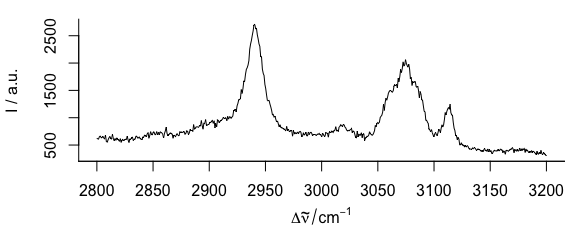

Figure 3.4: Spectra of paracetamol in range of 2800–3200 cm^-1.

By default, the values given are treated as wavelengths. If they are indices into the columns of the spectra matrix, use wl.index = TRUE:

plot(paracetamol[, , 2800:3200, wl.index = TRUE])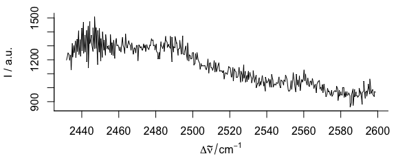

Figure 3.5: Spectra of paracetamol: from 2800^th to 3200^th point on wavelength axis.

Section 3.6.1 delves into the different possibilities of specifying wavelengths.

3.6.3 Deleting Wavelength Ranges

Deleting wavelength ranges may be accomplished using negative index vectors together with wl.index = TRUE.

plot(paracetamol[, , -(500:1000), wl.index = TRUE])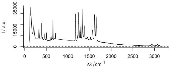

Figure 3.6: Spectra of paracetamol with 500^th to 1000^thwavelength axis point removed.

However, this mechanism works only if the proper indices are known.

If the range to be removed is instead specified in the units of the wavelength axis, it is easier to select the remainder of the spectrum instead. To delete the spectral range from 1750 to 2800 cm^-1 of the paracetamol spectrum one can use:

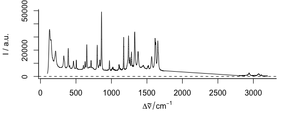
plot(paracetamol[, , c(min ~ 1750, 2800 ~ max)])

Figure 3.7: Spectra of paracetamol with range from 1750 to 2800 cm^-1 removed.

It is possible to produce a plot of this data where the cut range is actually omitted and the wavelength axis is optionally cut in order to save space. For details see the plotting vignette.

3.6.4 Changing the Wavelength Axis

Sometimes wavelength axes need to be transformed, e.g., converting from wavelengths to frequencies. In this case, retrieve the wavelength axis vector with wl(), convert each value of the resulting vector and assign the result with wl<-. Also the label of the wavelength axis may need to be adjusted.

As an example, convert the wavelength axis of laser to frequencies. As the wavelengths are in nanometers, and the frequencies are easiest expressed in terahertz, an additional conversion factor of 1000 is needed:

laser
#> hyperSpec object
#>    84 spectra
#>    3 data columns
#>    36 data points / spectrum

wavelengths <- wl(laser)
frequencies <- 2.998e8 / wavelengths / 1000
wl(laser) <- frequencies
labels(laser, ".wavelength") <- "f / THz"
laser
#> hyperSpec object
#>    84 spectra
#>    3 data columns
#>    36 data points / spectrum
rm(laser)

You can also accomplish these steps in a single line, e.g.,

wl(laser, "f / THz") <- frequencies

and

wl(laser) <- list(wl = frequencies, label = "f / THz")

see ?wl<- for more information.

3.6.5 Ordering the Wavelength Axis

If the wavelength axis of an object needs reordering (e.g., after collapse()), wl_sort() can be used:

barb <- collapse(barbiturates[1:3])
wl(barb)
#>  [1]  27.05  27.15  28.05  28.15  29.05  30.05  30.15  31.15  32.15  39.00  40.00  40.10  41.10
#> [14]  43.05  43.85  43.95  44.05  55.00  55.10  56.00  56.10  57.10  68.90  69.00  69.10  70.00
#> [27]  71.10  71.90  72.00  77.00  82.95  83.05  84.15  85.05  91.00  96.95  98.95 105.10 105.90
#> [40] 106.00 112.90 113.00 116.95 117.95 118.05 119.05 119.15 119.95 120.05 130.90 131.00 132.95
#> [53] 133.05 140.90 147.00 158.85 160.90

barb <- wl_sort(barb)
wl(barb)
#>  [1]  27.05  27.15  28.05  28.15  29.05  30.05  30.15  31.15  32.15  39.00  40.00  40.10  41.10
#> [14]  43.05  43.85  43.95  44.05  55.00  55.10  56.00  56.10  57.10  68.90  69.00  69.10  70.00
#> [27]  71.10  71.90  72.00  77.00  82.95  83.05  84.15  85.05  91.00  96.95  98.95 105.10 105.90
#> [40] 106.00 112.90 113.00 116.95 117.95 118.05 119.05 119.15 119.95 120.05 130.90 131.00 132.95
#> [53] 133.05 140.90 147.00 158.85 160.90

3.7 Conversion to Long- and Wide-Format `data.frame`s

Function as.data.frame() extracts the @data slot as a data.frame:

flu <- flu[, , 400 ~ 407] # make a small and handy version of the flu data set
as.data.frame(flu)
#>   spc.405 spc.405.5 spc.406 spc.406.5 spc.407         filename    c n .row
#> 1  27.150    32.345  33.379    34.419  36.531 rawdata/flu1.txt 0.05 1    1
#> 2  66.801    63.715  66.712    69.582  72.530 rawdata/flu2.txt 0.10 2    2
#> 3  93.144   103.068 106.194   110.186 113.249 rawdata/flu3.txt 0.15 3    3
#> 4 130.664   139.998 143.798   148.420 152.133 rawdata/flu4.txt 0.20 4    4
#> 5 167.267   171.898 177.471   184.625 189.752 rawdata/flu5.txt 0.25 5    5
#> 6 198.430   209.458 215.785   224.587 232.528 rawdata/flu6.txt 0.30 6    6

colnames(as.data.frame(flu))
#> [1] "spc"      "filename" "c"        "n"        ".row"

as.data.frame(flu)$spc
#>          405   405.5     406   406.5     407
#> [1,]  27.150  32.345  33.379  34.419  36.531
#> [2,]  66.801  63.715  66.712  69.582  72.530
#> [3,]  93.144 103.068 106.194 110.186 113.249
#> [4,] 130.664 139.998 143.798 148.420 152.133
#> [5,] 167.267 171.898 177.471 184.625 189.752
#> [6,] 198.430 209.458 215.785 224.587 232.528

Note that the spectra matrix is still a matrix inside column $spc.

Function as.data.frame() and the abbreviations $. and $.. retrieve the usual wide format data.frames:

flu$.
#>   spc.405 spc.405.5 spc.406 spc.406.5 spc.407         filename    c n
#> 1  27.150    32.345  33.379    34.419  36.531 rawdata/flu1.txt 0.05 1
#> 2  66.801    63.715  66.712    69.582  72.530 rawdata/flu2.txt 0.10 2
#> 3  93.144   103.068 106.194   110.186 113.249 rawdata/flu3.txt 0.15 3
#> 4 130.664   139.998 143.798   148.420 152.133 rawdata/flu4.txt 0.20 4
#> 5 167.267   171.898 177.471   184.625 189.752 rawdata/flu5.txt 0.25 5
#> 6 198.430   209.458 215.785   224.587 232.528 rawdata/flu6.txt 0.30 6

flu$..
#>           filename    c n
#> 1 rawdata/flu1.txt 0.05 1
#> 2 rawdata/flu2.txt 0.10 2
#> 3 rawdata/flu3.txt 0.15 3
#> 4 rawdata/flu4.txt 0.20 4
#> 5 rawdata/flu5.txt 0.25 5
#> 6 rawdata/flu6.txt 0.30 6

If another subset of colums needs to be extracted, use [[]]:

flu[[, c("c", "spc")]]
#>      c spc.405 spc.405.5 spc.406 spc.406.5 spc.407
#> 1 0.05  27.150    32.345  33.379    34.419  36.531
#> 2 0.10  66.801    63.715  66.712    69.582  72.530
#> 3 0.15  93.144   103.068 106.194   110.186 113.249
#> 4 0.20 130.664   139.998 143.798   148.420 152.133
#> 5 0.25 167.267   171.898 177.471   184.625 189.752
#> 6 0.30 198.430   209.458 215.785   224.587 232.528

This can be combined with extracting certain spectra and wavelengths, see 3.8.

The transpose of a wide format data.frame can be obtained by as.t.df(). For further examples, see the discussion of package ggplot2 in the plotting vignette.

as.t.df(apply(flu, 2, mean_pm_sd))
#>           .wavelength mean.minus.sd   mean mean.plus.sd
#> spc.405         405.0        49.958 113.91       177.86
#> spc.405.5       405.5        53.396 120.08       186.77
#> spc.406         406.0        55.352 123.89       192.43
#> spc.406.5       406.5        57.310 128.64       199.96
#> spc.407         407.0        59.513 132.79       206.06

Some functions need the data in an unstacked or long-format data.frame. Function as.long.df() is the appropriate conversion function.

head(as.long.df(flu), 20)
#>     .wavelength     spc         filename    c n
#> 1         405.0  27.150 rawdata/flu1.txt 0.05 1
#> 2         405.0  66.801 rawdata/flu2.txt 0.10 2
#> 3         405.0  93.144 rawdata/flu3.txt 0.15 3
#> 4         405.0 130.664 rawdata/flu4.txt 0.20 4
#> 5         405.0 167.267 rawdata/flu5.txt 0.25 5
#> 6         405.0 198.430 rawdata/flu6.txt 0.30 6
#> 1.1       405.5  32.345 rawdata/flu1.txt 0.05 1
#> 2.1       405.5  63.715 rawdata/flu2.txt 0.10 2
#> 3.1       405.5 103.068 rawdata/flu3.txt 0.15 3
#> 4.1       405.5 139.998 rawdata/flu4.txt 0.20 4
#> 5.1       405.5 171.898 rawdata/flu5.txt 0.25 5
#> 6.1       405.5 209.458 rawdata/flu6.txt 0.30 6
#> 1.2       406.0  33.379 rawdata/flu1.txt 0.05 1
#> 2.2       406.0  66.712 rawdata/flu2.txt 0.10 2
#> 3.2       406.0 106.194 rawdata/flu3.txt 0.15 3
#> 4.2       406.0 143.798 rawdata/flu4.txt 0.20 4
#> 5.2       406.0 177.471 rawdata/flu5.txt 0.25 5
#> 6.2       406.0 215.785 rawdata/flu6.txt 0.30 6
#> 1.3       406.5  34.419 rawdata/flu1.txt 0.05 1
#> 2.3       406.5  69.582 rawdata/flu2.txt 0.10 2

3.8 Conversion to Matrix

To obtain the spectral data as a matrix, simply use the [[]] extractor:

flu[[]]
#>          405   405.5     406   406.5     407
#> [1,]  27.150  32.345  33.379  34.419  36.531
#> [2,]  66.801  63.715  66.712  69.582  72.530
#> [3,]  93.144 103.068 106.194 110.186 113.249
#> [4,] 130.664 139.998 143.798 148.420 152.133
#> [5,] 167.267 171.898 177.471 184.625 189.752
#> [6,] 198.430 209.458 215.785 224.587 232.528

class(flu[[]])
#> [1] "matrix" "array"

Operator [[]] takes the same arguments as [], and can be used to extract a matrix containing parts of the spectra matrix:

flu[[1:3, , 406 ~ 407]]
#>          406   406.5     407
#> [1,]  33.379  34.419  36.531
#> [2,]  66.712  69.582  72.530
#> [3,] 106.194 110.186 113.249

If wavelengths or indices for the columns to extract are given, a data.frame is returned instead of a matrix:

flu[[1:3, c("filename", "spc"), 406 ~ 407]]
#>           filename spc.406 spc.406.5 spc.407
#> 1 rawdata/flu1.txt  33.379    34.419  36.531
#> 2 rawdata/flu2.txt  66.712    69.582  72.530
#> 3 rawdata/flu3.txt 106.194   110.186 113.249

4 Creating a hyperSpec Object, Data Import and Export

Package hyperSpec comes with filters for a variety of file formats. These are discussed in detail in a separate fileio vignette. Here we just mention a couple of basic operations.

4.1 Creating a `hyperSpec` Object from Spectra Matrix and Wavelength Vector

If the data is in R’s workspace, a hyperSpec object is created by:

spc <- new("hyperSpec", spc = spectra.matrix, wavelength = wavelength.vector, data = extra.data)

The most frequently needed arguments are:

`spc`	The spectra matrix; may be a matrix or a `data.frame`.
`wavelength`	The wavelength axis as a numeric vector.
`data`	Any extra data as a `data.frame`. It is possible to pass `spc` via this argument if the data frame has a column `$spc`.
`label`	A list with the proper labels. Do not forget the wavelength axis label in `$.wavelength` and the spectral intensity axis label in `$spc`.

More information about converting existing data into hyperSpec objects can be found in the fileio vignette.

4.2 Creating Random Spectra

If package mvtnorm[1,2] is available, multivariate normally distributed spectra can be generated from mean and covariance matrix using rmmvnorm() (Fig. 4.1). Note that the package hyperSpec function’s name has an additional “m”: it already takes care of multiple groups. Mean spectra and pooled covariance matrix can be calculated using pooled.cov():

pcov <- pooled.cov(faux_cell, faux_cell$region)
rnd <- rmmvnorm(rep(10, 3), mean = pcov$mean, sigma = pcov$COV)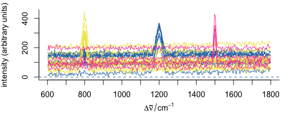

cluster.cols <- palette_colorblind[c(2, 7, 4)]
plot(rnd, col = cluster.cols[rnd$.group])

Multivariate normally distributed random spectra generated with `rmmvnorm()`{.r}.

Figure 4.1: Multivariate normally distributed random spectra generated with rmmvnorm().

5 Spectral Pre-Processing

5.1 Cutting the Spectral Range

Please refer to Table 3.1, Table 3.2 and Section 3.6 for information and examples of cutting the spectral range.

5.2 Shifting Spectra

Sometimes, spectra need to be aligned along the spectral axis.

In general, two options are available for shifting spectra along the wavelength axis.

The wavelength axis can be shifted, while the intensities stay unaffected.
The spectra are interpolated onto a new wavelength axis, while the nominal wavelengths stay.

The first method is very straightforward (Fig. 5.1):

tmp <- faux_cell
wl(tmp) <- wl(tmp) - 10

plot(faux_cell[135])
plot(tmp[135, , ], add = TRUE, col = palette_colorblind[4])

Figure 5.1: Shifting the spectra along the wavelength axis: changing the wavelength values.

But the method cannot be used if each spectrum (or groups of spectra) are shifted individually. In that case, interpolation is needed. R offers many possibilities to interpolate (e.g., approx() for constant / linear approximation, spline() for spline interpolation, loess() can be used to obtain smoothed approximations, etc.). The appropriate interpolation strategy will depend on the spectra, and package hyperSpec therefore leaves it up to the user to select a sensible interpolation function.

As an example, we will use natural splines to do the interpolation. It is convenient to set it up as a function:

interpolate <- function(spc, shift, wl) {
  spline(wl + shift, spc, xout = wl, method = "natural")$y
}

This function can now be applied to a set of spectra (Fig. 5.2):

tmp <- apply(faux_cell, 1, interpolate, shift = -10, wl = wl(faux_cell))

plot(faux_cell[135])
plot(tmp[135], add = TRUE, col = palette_colorblind[4])

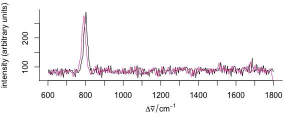
Figure 5.2: Shifting the spectra along the wavelength axis: interpolation.

Fig. 5.3 demonstrates the difference between simple shifting and interpolation.

tmp <- faux_cell[135, , 990 ~ 1010]
plot(tmp, lines.args = list(type = "b", pch = 19, cex = 0.5))
wl(tmp) <- wl(tmp) - 0.5
plot(tmp, lines.args = list(type = "b", pch = 19, cex = 0.5), add = TRUE, col = palette_colorblind[4])

tmp <- faux_cell[135]
tmp <- apply(tmp, 1, function(x, wl, shift) {
  spline(wl + shift, x, xout = wl)$y
},
wl = wl(tmp), shift = -0.5
)
plot(tmp, lines.args = list(type = "b", pch = 19, cex = 0.5), add = TRUE, col = palette_colorblind[3])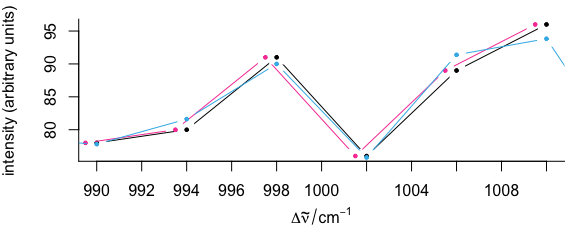

Shifting the spectra along the wavelength axis.
Detail view of the phenylalanine band: shifting by `wl<-`{.r} (red) does not affect the intensities, while the spectrum is slightly changed by interpolations (blue).

Figure 5.3: Shifting the spectra along the wavelength axis. Detail view of the phenylalanine band: shifting by wl<- (red) does not affect the intensities, while the spectrum is slightly changed by interpolations (blue).

If different spectra need to be offset by different shift, use a loop².

shifts <- rnorm(nrow(faux_cell))
tmp <- faux_cell[[]]
for (i in seq_len(nrow(faux_cell))) {
  tmp[i, ] <- interpolate(tmp[i, ], shifts[i], wl = wl(faux_cell))
}
faux_cell[[]] <- tmp

5.2.1 Calculating the Shift

Often, the shift in the spectra is determined by aligning a particular signal. This strategy works best with spectrally oversampled data that allows accurate determination of the signal position.

For the faux_cell data, let’s use the maximum of the peak around 1200 cm^-1. As just the very maximum is too coarse, we’ll use the maximum of a square polynomial fitted to the maximum and its two neighbours.

# FIXME: this code currently does not work.
find_max <- function(y, x) {
  pos <- which.max(y) + (-1:1)
  X <- x[pos] - x[pos[2]]
  Y <- y[pos] - y[pos[2]]

  X <- cbind(1, X, X^2)
  coef <- qr.solve(X, Y)

  -coef[2] / coef[3] / 2 + x[pos[2]]
}

bandpos <- apply(faux_cell[[, , 1190 ~ 1210]], 1, find_max, wl(faux_cell[, , 1190 ~ 1210]))
refpos <- find_max(colMeans(faux_cell[[, , 1190 ~ 1210]]), wl(faux_cell[, , 1190 ~ 1210]))

shift1 <- refpos - bandpos

A second possibility is to optimize the shift. For this strategy, the spectra must be sufficiently similar, while low spectral resolution is compensated by using larger spectral windows.

faux_cell_tmp <- faux_cell - spc_fit_poly_below(faux_cell[, , min + 3i ~ max - 3i], faux_cell)
faux_cell_tmp <- sweep(faux_cell_tmp, 1, rowMeans(faux_cell[[]], na.rm = TRUE), "/")

targetfn <- function(shift, wl, spc, targetspc) {
  error <- spline(wl + shift, spc, xout = wl)$y - targetspc
  sum(error^2)
}

shift2 <- numeric(nrow(faux_cell))
tmp <- faux_cell[[]]
target <- colMeans(faux_cell[[]])
for (i in 1:nrow(faux_cell)) {
  shift2[i] <- unlist(optimize(targetfn,
    interval = c(-5, 5),
    wl = faux_cell@wavelength,
    spc = tmp[i, ], targetspc = target
  )$minimum)
}

Figure ?? shows that the second correction method works better for the faux_cell data. This was expected, as the spectra are hardly or not oversampled, but are very similar to each other.

# FIXME: this code currently does not work.
df <- data.frame(
  shift = c(shifts, shifts + shift1, shifts + shift2),
  method = rep(c("original", "find maximum", "interpolation"),
    each = nrow(faux_cell)
  )
)
plot(histogram(~ shift | method,
  data = df, breaks = do.breaks(range(df$shift), 25),
  layout = c(3, 1)
))

5.3 Removing Bad Data

5.3.1 Bad Spectra

Occasionally, one may want to remove spectra because of too low or too high signal. E.g., for infrared spectra one may state that the absorbance maximum should be, say, between 0.1 and 1. Class hyperSpec’s comparison operators return a logical matrix of the size of the spectra that is suitable for later indexing:

ir_spc <- faux_cell / 1500 ## fake IR data
high_int <- apply(ir_spc > 1, 1, any) # any point above 1 is bad
low_int <- apply(ir_spc, 1, max) < 0.1 # the maximum should be at least 0.1
ir_spc <- ir_spc[!high_int & !low_int]

5.3.2 Removing Spectra Outside Mean $\pm$ $n$ Standard Deviations

mean_sd_filter <- function(x, n = 5) {
  x <- x - mean(x)
  s <- n * sd(x)
  (x <= s) & (x > -s)
}

OK <- apply(faux_cell[[]], 2, mean_sd_filter, n = 4) # logical matrix

spc.OK <- faux_cell[apply(OK, 1, all)]

plot(faux_cell[!apply(OK, 1, all)])
i <- which(!OK, arr.ind = TRUE)
points(wl(faux_cell)[i[, 2]], faux_cell[[!OK]], pch = 19, col = palette_colorblind[4], cex = 0.5)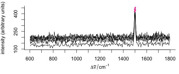

$Filtering data: mean $\pm$ sd filter.$

Figure 5.4: Filtering data: mean $\pm$ sd filter.

5.3.3 Bad Data Points

Assume the data occasionally has a detector readout of 0:

spc <- faux_cell[1:3, , min ~ min + 15i]
spc[[cbind(1:3, sample(nwl(spc), 3)), wl.index = TRUE]] <- 0
spc[[]]
#>         602     606     610     614    618     622     626    630     634     638     642     646
#> [1,] 138.13 129.659 138.745 144.504 131.23 136.949 111.078 124.11 123.946   0.000 126.461 136.325
#> [2,]   0.00  73.371  99.227  83.301  54.00  74.184  68.029  79.00  73.236  98.166  82.623  73.986
#> [3,] 120.10 132.189   0.000 117.864 125.13 122.796 111.221 146.10 121.732 123.221 142.052 137.024
#>          650     654     658     662
#> [1,] 142.723 150.316 140.794 125.848
#> [2,]  72.874  69.232  90.187  83.842
#> [3,] 140.820 113.921 127.047 120.082

We can set these points to NA, again using that the comparison returns a suitable logical matrix:

spc[[spc < 1e-4]] <- NA
spc[[]]
#>         602     606     610     614    618     622     626    630     634     638     642     646
#> [1,] 138.13 129.659 138.745 144.504 131.23 136.949 111.078 124.11 123.946      NA 126.461 136.325
#> [2,]     NA  73.371  99.227  83.301  54.00  74.184  68.029  79.00  73.236  98.166  82.623  73.986
#> [3,] 120.10 132.189      NA 117.864 125.13 122.796 111.221 146.10 121.732 123.221 142.052 137.024
#>          650     654     658     662
#> [1,] 142.723 150.316 140.794 125.848
#> [2,]  72.874  69.232  90.187  83.842
#> [3,] 140.820 113.921 127.047 120.082

Depending on the type of analysis, one may wish to replace the NAs by interpolating the neighbour values. Package hyperSpec provides three functions that can interpolate the NAs: spc_na_approx(), spc_loess(), and spc_bin() with na.rm = TRUE (the latter two are discussed below).

spc.corrected <- spc_na_approx(spc)
spc.corrected[[]]
#>          602     606     610     614    618     622     626    630     634     638     642     646
#> [1,] 138.127 129.659 138.745 144.504 131.23 136.949 111.078 124.11 123.946 125.204 126.461 136.325
#> [2,]  73.371  73.371  99.227  83.301  54.00  74.184  68.029  79.00  73.236  98.166  82.623  73.986
#> [3,] 120.105 132.189 125.026 117.864 125.13 122.796 111.221 146.10 121.732 123.221 142.052 137.024
#>          650     654     658     662
#> [1,] 142.723 150.316 140.794 125.848
#> [2,]  72.874  69.232  90.187  83.842
#> [3,] 140.820 113.921 127.047 120.082

spc[[is.na(spc)]] <- 0
plot(spc)

spc[[spc < 1e-4]] <- NA
plot(spc_na_approx(spc),
  add = TRUE, col = palette_colorblind[4],
  lines.args = list(type = "b", pch = 19, cex = 0.5)
)

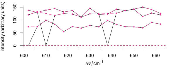
Figure 5.5: Filtering data: remove bad points.

5.3.4 Spikes in Raman Spectra

Correction of cosmic spikes is not a part of hyperSpec package, but can be addressed with algorithms presented in these papers:

5.4 Smoothing Interpolation

Spectra acquired by grating instruments are frequently interpolated onto a new wavelength axis, e.g., because the unequal data point spacing should be removed. Also, the spectra can be smoothed: reducing the spectral resolution allows to increase the signal to noise ratio. For chemometric data analysis reducing the number of data points per spectrum may be crucial as it reduces the dimensionality of the data. Package hyperSpec provides two functions to do so: spc_bin() and spc_loess().

Function spc_bin() bins the spectral axis by averaging every by data points.

plot(paracetamol, wl.range = c(300 ~ 1800, 2800 ~ max), xoffset = 850)
#> Loading required namespace: plotrix
p <- spc_loess(paracetamol, c(seq(300, 1800, 2), seq(2850, 3150, 2)))
plot(p, wl.range = c(300 ~ 1800, 2800 ~ max), xoffset = 850, col = palette_colorblind[4], add = TRUE)

b <- spc_bin(paracetamol, 4)
plot(b,
  wl.range = c(300 ~ 1800, 2800 ~ max), xoffset = 850,
  lines.args = list(pch = 20, cex = .3, type = "p"), col = palette_colorblind[3], add = TRUE
)

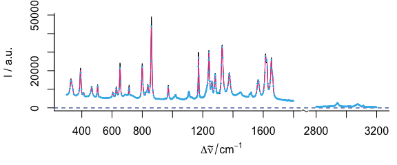
$Smoothing interpolation by `spc_loess()`{.r} with new data point spacing of 2 cm^-1^ (red) and `spc_bin()`{.r} (blue).$

Figure 5.6: Smoothing interpolation by spc_loess() with new data point spacing of 2 cm^-1 (red) and spc_bin() (blue).

plot(paracetamol[, , 1600 ~ 1670])
plot(p[, , 1600 ~ 1670], col = palette_colorblind[4], add = TRUE)
plot(b[, , 1600 ~ 1670], col = palette_colorblind[3], add = TRUE)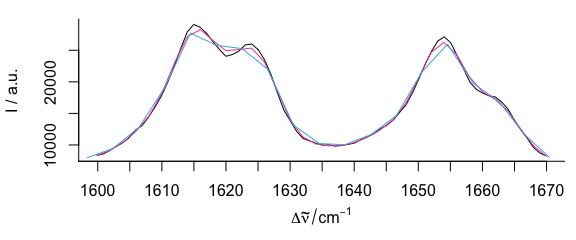

$The magnification of Fig. \@ref(fig:fig-loess) shows how interpolation may cause a loss in signal height.$

Figure 5.7: The magnification of Fig. 5.6 shows how interpolation may cause a loss in signal height.

Function spc_loess() applies R’s loess() function for spectral interpolation. Figures 5.6 and 5.7 show the result of interpolating from 300 to 1800 and 2850 to 3150 cm^-1 with 2 cm^-1 data point distance. This corresponds to a spectral resolution of about 4 cm^-1, and the decrease in spectral resolution can be seen at the sharp bands where the maxima are not reached (due to the fact that the interpolation wavelength axis does not necessarily hit the maxima. The original spectrum had 4064 data points with unequal data point spacing (between 0 and 1.4 cm^-1). The interpolated spectrum has 902 data points.

5.5 Background Correction

To subtract a background spectrum of each of the spectra in an object, use:

sweep(spectra, 2, background.spectrum, "-")

5.6 Offset Correction

Calculate the offsets and adjust the spectra accordingly:

offsets <- apply(faux_cell, 1, min)
faux_cell_offset_corrected <- sweep(faux_cell, 1, offsets, "-")

If the offset is calculated by a function, as here with the min(), hyperSpec’s sweep() method offers a shortcut: sweep()’s STATS argument may be the function instead of a numeric vector:

faux_cell_offset_corrected <- sweep(faux_cell, 1, min, "-")

5.7 Baseline Correction

Package hyperSpec comes with two functions to fit polynomial baselines.

Functions spc_fit_poly_below(), spc_fit_poly() fit a polynomial baseline of the given order. A least-squares fit is done so that the function may be used on rather noisy spectra. However, the user must supply an object that is cut appropriately. Particularly, the supplied wavelength ranges are not weighted.

Function spc_fit_poly_below() tries to find appropriate support points for the baseline iteratively.

Both functions return a hyperSpec object containing the fitted baselines. They need to be subtracted afterwards:

bl <- spc_fit_poly_below(faux_cell)
faux_cell_tmp <- faux_cell - bl

For details, see baseline vignette.

Package package baseline[3,4] offers many more functions for baseline correction. The baseline() function works on the spectra matrix, which is extracted by [[]]. The result is a baseline object, but can easily be re-imported into the hyperSpec object:

corrected <- hyperSpec::faux_cell[1] # start with the unchanged data set

library("baseline")
#> 
#> Attaching package: 'baseline'
#> The following object is masked from 'package:pls':
#> 
#>     mvrValstats
#> The following object is masked from 'package:stats':
#> 
#>     getCall
bl <- baseline(corrected[[]], method = "modpolyfit", degree = 4)
corrected[[]] <- getCorrected(bl)

Fig. 5.8 and 5.9 show raw data and the result for the first spectrum of faux_cell.

baseline <- corrected
baseline[[]] <- getBaseline(bl)
plot(hyperSpec::faux_cell[1], plot.args = list(ylim = range(hyperSpec::faux_cell[1], 0)))
plot(baseline, add = TRUE, col = palette_colorblind[4])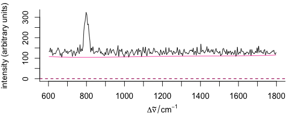

$The first spectrum of `faux_cell`{.r} (raw data) with baseline.$

Figure 5.8: The first spectrum of faux_cell (raw data) with baseline.

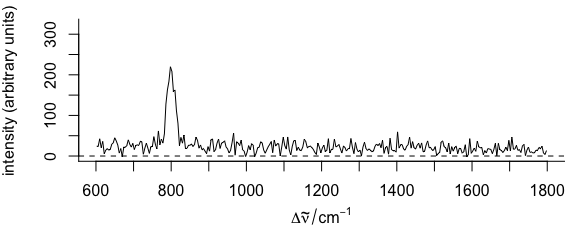
plot(corrected, plot.args = list(ylim = range(hyperSpec::faux_cell[1], 0)))

$Baseline correction using the **baseline** package: the first spectrum of `faux_cell`{.r} after baseline correction with method "odpolyfi".$

Figure 5.9: Baseline correction using the baseline package: the first spectrum of faux_cell after baseline correction with method “odpolyfi”.

rm(bl, faux_cell)

5.8 Intensity Calibration

5.8.1 Correcting by a Constant, e. g. Readout Bias

CCD cameras often operate with a bias, causing a constant value for each pixel. Such a constant can be immediately subtracted: spectra - constant.

5.8.2 Correcting Wavelength Dependence

For each of the wavelengths the same correction needs to be applied to all spectra.

There might be wavelength dependent offsets (background or dark spectra). They are subtracted:
```
sweep(spectra, 2, offset.spectrum, "-")
```
A multiplicative dependency such as a CCD’s photon efficiency:
```
sweep(spectra, 2, photon.efficiency, "/")
```

5.8.3 Spectra Dependent Correction

If the correction depends on the spectra (e. g. due to inhomogeneous illumination while collecting imaging data, differing optical path length, etc.), the MARGIN of the sweep() function needs to be 1 or SPC:

Pixel dependent offsets are subtracted:
```
sweep(spectra, SPC, pixel.offsets, "-")
```

A multiplicative dependency:

sweep(spectra, SPC, illumination.factors, "*")

5.9 Normalization

Again, sweep() is the function of choice. E.g., for area normalization, use:

faux_cell_tmp <- sweep(faux_cell, 1, mean, "/")

(Using the mean instead of the sum results in conveniently scaled spectra with intensities around 1.)

If the calculation of the normalization factors is more elaborate, use a two step procedure:

Calculate appropriate normalization factors You may calculate the factors using only a certain wavelength range, thereby normalizing on a particular band or peak.

Again, sweep the factor off the spectra:

normalized <- sweep(spectra, 1, factors, "*")

factors <- 1 / apply(faux_cell[, , 1600 ~ 1700], 1, mean)
faux_cell_tmp <- sweep(faux_cell, 1, factors, "*")

For the special case of area normalization using the mean spectra, the factors can be more conveniently calculated by

factors <- 1 / rowMeans(faux_cell[, , 1600 ~ 1700])

and instead of sweep the arithmetic operators (here *) can be used directly with the normalization factor:

faux_cell_tmp <- faux_cell * factors

Put together, this results in:

faux_cell_tmp <- faux_cell / rowMeans(faux_cell[, , 1600 ~ 1700])

For minimum-maximum-normalization, first do an offset- or baseline correction, then normalize using max().

5.10 Centering and Variance Scaling the Spectra

Centering means that the mean spectrum is subtracted from each of the spectra. Many data analysis techniques, like principal component analysis, partial least squares, etc., work much better on centered data. From a spectroscopic point of view it depends on the particular data set whether centering does make sense or not.

Variance scaling is often used in multivariate analysis to adjust the influence and scaling of the variates (that are typically different physical values). However, spectra already do have the same scale of the same physical value. Thus one has to trade off the the expected numeric benefit with the fact that for wavelengths with low signal the noise level will greatly increase when using variance scaling. Scaling usually makes sense only for centered data.

Both tasks are carried out by the same method in R, scale(), which will by default both mean center and variance scale the spectra matrix.

To center the flu data set, use:

flu.centered <- scale(flu, scale = FALSE)
plot(flu.centered)

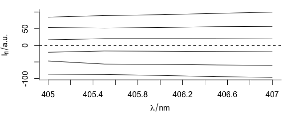
Figure 5.10: Mean-centered spectra of flu.

On the other hand, the faux_cell data set consists of Raman spectra, so the spectroscopic interpretation of centering is getting rid of the the average chemical composition of the sample. But what is the meaning of the “Average spectrum” of an inhomogeneous sample? In this case it may be better to subtract the minimum spectrum (which will hopefully have almost the same benefit on the data analysis) as it is the spectrum of that chemical composition that is underlying the whole sample.

One more point to consider is that the actual minimum spectrum will pick up (negative) noise. In order to avoid that, using, e.g., the 5^th percentile spectrum is more suitable:

faux_cell_tmp <- scale(faux_cell, center = quantile(faux_cell, 0.05), scale = FALSE)
plot(faux_cell_tmp, "spcprctl5")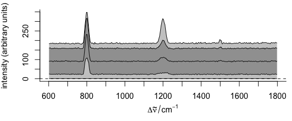

Figure 5.11: The summary spectra of faux_cell with 5^th percentile subtracted.

See section the appendices for some tips to speed up these calculations.

5.11 Multiplicative Scatter Correction

Multiplicative scatter correction (MSC) can be done using msc() from package package pls [5]. It operates on the spectra matrix:

library(pls)
faux_cell_msc <- faux_cell
faux_cell_msc[[]] <- msc(faux_cell[[]])

5.12 Spectral Arithmetic

Basic mathematical functions are defined for hyperSpec objects. You may convert spectra to their log:

absorbance.spectra <- -log10(transmission.spectra)

In this case, do not forget to adapt the label:

labels(absorbance.spectra)$spc <- "A"

Be careful: R’s log() function calculates the natural logarithm if no base is given.

The basic arithmetic operators work element-wise in R. Thus they all need either a scalar, or a matrix (or hyperSpec object) of the correct size.

Matrix multiplication is done by %*%, again each of the operands may be a matrix or a hyperSpec object, and must have the correct dimensions.

There are many more mathematical functions that understand a hyperSpec object. See ?Arith for more details.

6 Data Analysis

6.1 Principal Component Analysis with `prcomp()`

6.1.1 Carrying out PCA

The $. notation is handy, if a data analysis function expects a data.frame, as prcomp() does. The column names can then be used in the formula:

pca <- prcomp(~spc, data = faux_cell$., center = FALSE)

However, many modeling functions call as.data.frame on their data argument, including prcomp(). In that case, the conversion is done automatically so the following gives the same result as above:

pca <- prcomp(~spc, data = faux_cell, center = FALSE)

6.1.2 Plotting the Results of PCA

The results of such a decomposition can be put back into hyperSpec objects. This conveniently allows one to use the regular hyperSpec plotting functions, e.g., the loading-like spectra, or score maps, see Figures 6.1 and 6.2.

scores <- decomposition(faux_cell, pca$x,
  label.wavelength = "PC",
  label.spc = "score / a.u."
)
scores
#> hyperSpec object
#>    875 spectra
#>    4 data columns
#>    300 data points / spectrum

The loadings can be similarly re-imported:

loadings <- decomposition(faux_cell, t(pca$rotation),
  scores = FALSE,
  label.spc = "loading I / a.u."
)
loadings
#> hyperSpec object
#>    300 spectra
#>    1 data columns
#>    300 data points / spectrum

There is, however, one important difference. The loadings are thought of as values computed from all spectra together. Thus no meaningful extra data can be assigned for the loadings object (at least not if the column consists of different values). Therefore, the loadings object lost all extra data (see above).

Argument retain.columns triggers whether columns that contain different values should be dropped. If it is set to TRUE, the columns are retained, but contain NAs:

loadings <- decomposition(faux_cell, t(pca$rotation),
  scores = FALSE,
  retain.columns = TRUE, label.spc = "loading I / a.u."
)
loadings[1]$..
#>      x  y region
#> PC1 NA NA   <NA>

If an extra data column does contain only one unique value, it is retained regardless:

faux_cell$measurement <- 1
loadings <- decomposition(faux_cell, t(pca$rotation),
  scores = FALSE,
  label.spc = "loading I / a.u."
)
loadings[1]$..
#>     measurement
#> PC1           1

plot(loadings[1:3], stacked = TRUE)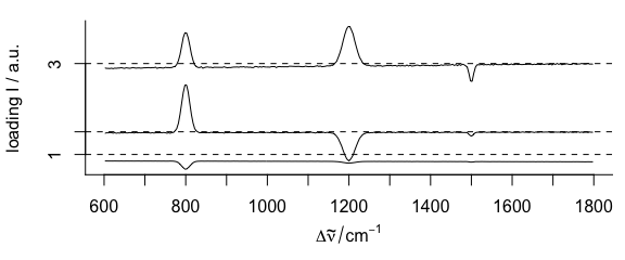

Figure 6.1: The first three loadings.

div_palette <- colorRampPalette(c(
  "#00008B", "#351C96", "#5235A2", "#6A4CAE", "#8164BA", "#967CC5",
  "#AC95D1", "#C1AFDC", "#D5C9E8", "#E0E3E3", "#F8F8B0", "#F7E6C2",
  "#EFCFC6", "#E6B7AB", "#DCA091", "#D08977", "#C4725E", "#B75B46",
  "#A9432F", "#9A2919", "#8B0000"
), space = "Lab")

plotmap(scores[, , 3], col.regions = diverging_hcl(20, palette = "Blue-Red2"))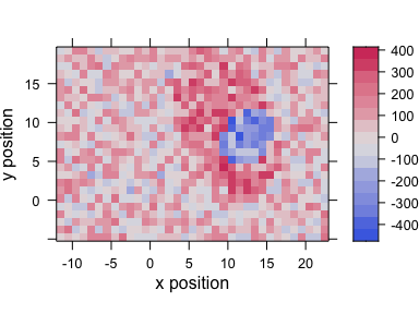

Figure 6.2: The third score map.

6.1.3 PCA as Noise Filter

Principal component analysis is sometimes used as a noise filtering technique. The idea is that the relevant differences are captured in the first few components while the higher components contain noise only. Thus the spectra are reconstructed using only the first $p$ components.

This reconstruction is in fact a matrix multiplication:

\[\begin{equation} \mathrm{spectra}^{\mathrm{~nrow} ~×~ \mathrm{nwl}} = \mathrm{scores}^{\mathrm{~nrow} ~×~ p} \;\cdot\; \mathrm{loadings}^{~p ~×~ \mathrm{nwl}} \tag{6.1} \end{equation}\]

Note that this corresponds to a model based on the Beer-Lambert law: \[\begin{equation} A_n (\lambda) = c_{n,i} \epsilon (i, \lambda) + \mathrm{error} \tag{6.2} \end{equation}\] The matrix formulation puts the $n$ spectra into the rows of $A$ and $c$, while the $i$ pure components appear in the columns of $c$ and rows of the absorbance coefficients $\epsilon$.

For an ideal data set (constituents varying independently, sufficient signal to noise ratio) one would expect the principal component analysis to extract something like the concentrations and pure component spectra.

If we decide that only the first 10 components actually carry spectroscopic information, we can reconstruct spectra with better signal to noise ratio:

smoothed <- scores[, , 1:10] %*% loadings[1:10]

Keep in mind, though, that we cannot be sure how much useful information was discarded with the higher components. This kind of noise reduction may influence further modeling of the data. Mathematically speaking, the rank of the new 875 $×$ 300 spectra matrix is only 10.

6.2 Hierarchical Cluster Analysis

Some R functions expect their input data in a matrix, including those related to HCA. Conveniently, the [[]] extraction function returns a matrix.

dist <- pearson.dist(faux_cell[[]])

Again, many such functions coerce the data to a matrix automatically, so the hyperSpec object can be handed over without the explicit conversion above (as we saw for PCA):

dist <- pearson.dist(faux_cell)
dendrogram <- hclust(dist, method = "ward.D")

plot(dendrogram, labels = FALSE, hang = -1)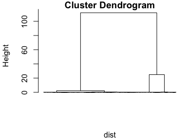

Figure 6.3: The results of the cluster analysis: the dendrogram.

In order to plot a cluster map, the cluster membership needs to be calculated from the dendrogram.

First, cut the dendrogram so that three clusters result:

faux_cell$region <- as.factor(cutree(dendrogram, k = 3))

As the cluster membership was stored as factor, the levels can be meaningful names, which are displayed in the color legend.

levels(faux_cell$region) <- c("matrix", "lacuna", "cell")

Then the result may be plotted (Figure 6.4):

plotmap(faux_cell, region ~ x * y, col.regions = cluster.cols)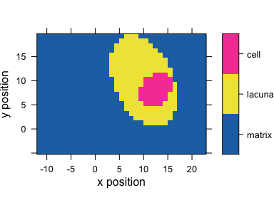

Figure 6.4: The results of the cluster analysis: the map of the 3 clusters.

6.3 Calculating Group-Wise Sum Characteristics, e. g. Cluster Mean Spectra

Function aggregate() applies the function given in FUN to each of the groups of spectra specified in by.

So we may plot the cluster mean spectra:

means <- aggregate(faux_cell, by = faux_cell$region, mean_pm_sd)
plot(means, col = cluster.cols, stacked = ".aggregate", fill = ".aggregate")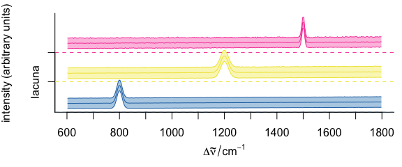

Figure 6.5: The results of the cluster analysis: the the mean spectra.

7 Combining and Splitting `hyperSpec` Objects

7.1 Binding Objects Together

Class hyperspec objects can be bound together, either by columns (cbind()) to append a new spectral range or by row (rbind()) to append new spectra:

dim(flu)
#> nrow ncol  nwl 
#>    6    4    5

dim(cbind(flu, flu))
#> nrow ncol  nwl 
#>    6    4   10

dim(rbind(flu, flu))
#> nrow ncol  nwl 
#>   12    4    5

There is also a more general function, bind(), taking the direction ("r" or "c") as first argument followed by the objects to bind either in separate arguments or in a list.

As usual for rbind() and cbind(), the objects that should be bound together must have the same number of columns (for rbind()) and the same number of rows (for cbind()), respectively.

For binding row-wise (rbind()), collapse() is more flexible and faster as well.

7.2 Binding Objects that Do not Share the Same Extra Data and/or Wavelength Axis

Function collapse() combines objects that should be bound together by row, but they do not share the columns and/or spectral range. The resulting object has all columns from all input objects, and all wavelengths from the input objects. If an input object does not have a particular column or wavelength, its value in the resulting object is NA.

The barbiturates data is a list of 5 hyperSpec objects, each containing one mass spectrum. The spectra have between 22 and 37 data points each.

barb <- collapse(barbiturates)
wl(barb)[1:25]
#>  [1] 27.05 27.15 28.05 28.15 29.05 30.05 30.15 31.15 32.15 38.90 39.00 40.00 40.10 41.10 43.05 43.85
#> [17] 43.95 44.05 55.00 55.10 56.00 56.10 57.00 57.10 68.90

The resulting object does not have an ordered wavelength axis. This can be obtained in the second step:

barb <- wl_sort(barb)
barb[[1:3, , min ~ min + 10i]]
#>      27.05 27.15 28.05 28.15 29.05 30.05 30.15 31.15 32.15 38.9  39
#> [1,]   562    NA    NA 11511  6146  1253    NA  9851 10751   NA 756
#> [2,]    NA   618 10151    NA  5040    NA   910  8200 10989   NA 770
#> [3,]   638    NA    NA 10722  5253   966    NA  8709 10899   NA  NA

7.3 Binding Objects that Do not Share the Same Spectra

Function merge() adds a new spectral range (like cbind()), but works also if spectra are missing in one of the objects. The arguments by, by.x, and by.y specify which columns should be used to decide which spectra are the same. The arguments all, all.x, and all.y determine whether spectra should be kept for the result set if they appear in only one of the objects. For details, see also the help on the base function merge().

As an example, let’s construct a version of the faux_cell data like being taken as two maps with different spectral ranges. In each data set, some spectra are missing.

faux_cell_low <- sample(faux_cell[, , min ~ 1200], 700)
nrow(faux_cell_low)
#> [1] 700

faux_cell_high <- sample(faux_cell[, , 1400 ~ max], 700)
nrow(faux_cell_high)
#> [1] 700

As all extra data columns are the same, no special declarations are needed for merging the data:

faux_cell_merged <- merge(faux_cell_low, faux_cell_high)
nrow(faux_cell_merged)
#> [1] 559

By default, the result consists of only those spectra, where both spectral ranges were available. To keep all spectra replacing missing parts by NA (see Fig. 7.1, 7.2):

faux_cell_merged <- merge(faux_cell_low, faux_cell_high, all = TRUE)
nrow(faux_cell_merged)
#> [1] 841

matcols <- sequential_hcl(20, palette = "viridis")
levelplot(spc ~ x * y | as.factor(paste(.wavelength, "  1/cm")),
  faux_cell_merged[, , c(1000, 1650)],
  aspect = "iso", col.regions = matcols
)

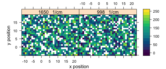
Figure 7.1: For both spectral ranges some spectra are missing.

plot(faux_cell_merged[1:100], "mat", col = matcols)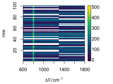

The missing parts of the spectra are filled with `NA`{.r}.

Figure 7.2: The missing parts of the spectra are filled with NA.

merged <- merge(faux_cell[1:7, , 610 ~ 620], faux_cell[5:10, , 615 ~ 625], all = TRUE)
merged$.
#>         x     y region measurement .nx .ny spc.1 spc.2 spc.3 spc.4 spc.5 spc.6 spc.7
#> 1  -11.55 -4.77 matrix           1   1  NA   150   128   143    NA    NA    NA    NA
#> 2  -10.55 -4.77 matrix           1   2  NA    99    84    54    NA    NA    NA    NA
#> 3   -9.55 -4.77 matrix           1   3  NA   142   118   125    NA    NA    NA    NA
#> 4   -8.55 -4.77 matrix           1   4  NA    83   108   126    NA    NA    NA    NA
#> 5   -7.55 -4.77 matrix           1   5   1    27    19    23    19    23    27    31
#> 6   -6.55 -4.77 matrix           1   6   2    14    18    12    18    12    20    17
#> 7   -5.55 -4.77 matrix           1   7   3    22    24    23    24    23    28    31
#> 8   -4.55 -4.77 matrix           1  NA   4    NA    NA    NA    74    78    86    81
#> 9   -3.55 -4.77 matrix           1  NA   5    NA    NA    NA     0     0     0     1
#> 10  -2.55 -4.77 matrix           1  NA   6    NA    NA    NA   122   129   135   119

If the spectra overlap, the result will have both data points. In the example here one could easily delete duplicate wavelengths. For real data, however, the duplicated wavelength will hardly ever contain the same values. The appropriate method to deal with this situation depends on the data at hand, but it will usually be some kind of spectral interpolation.

One possibility is removing duplicated wavelengths by using the mean intensity. This can conveniently be done by using approx() using method = "constant". For duplicated wavelengths, the intensities will be combined by the tie function. This already defaults to the mean, but we need na.rm = TRUE.

Thus, the function to calculate the new spectral intensities is

approxfun <- function(y, wl, new.wl) {
  approx(wl, y, new.wl,
    method = "constant",
    ties = function(x) mean(x, na.rm = TRUE)
  )$y
}

which can be applied to the spectra:

merged <- apply(merged, 1, approxfun,
  wl = wl(merged),
  new.wl = unique(wl(merged)),
  new.wavelength = "new.wl"
)
merged$.
#>         x     y region measurement .nx .ny spc.1 spc.2 spc.3 spc.4 spc.5
#> 1  -11.55 -4.77 matrix           1   1  NA   150   128   143    NA    NA
#> 2  -10.55 -4.77 matrix           1   2  NA    99    84    54    NA    NA
#> 3   -9.55 -4.77 matrix           1   3  NA   142   118   125    NA    NA
#> 4   -8.55 -4.77 matrix           1   4  NA    83   108   126    NA    NA
#> 5   -7.55 -4.77 matrix           1   5   1    27    19    23    27    31
#> 6   -6.55 -4.77 matrix           1   6   2    14    18    12    20    17
#> 7   -5.55 -4.77 matrix           1   7   3    22    24    23    28    31
#> 8   -4.55 -4.77 matrix           1  NA   4    NA    74    78    86    81
#> 9   -3.55 -4.77 matrix           1  NA   5    NA     0     0     0     1
#> 10  -2.55 -4.77 matrix           1  NA   6    NA   122   129   135   119

7.4 Merging Extra Data to Objects That Do Not (Necessarily) Share the Same Spectra

Assume we obtained duplicate reference measurements for some of the concentrations in flu:

flu.ref <- data.frame(
  filename = rep(flu$filename[1:2], each = 2),
  cref     = rep(flu$c[1:2], each = 2) + rnorm(4, sd = 0.01)
)
flu.ref
#>           filename     cref
#> 1 rawdata/flu1.txt 0.044329
#> 2 rawdata/flu1.txt 0.044622
#> 3 rawdata/flu2.txt 0.087589
#> 4 rawdata/flu2.txt 0.119215

This information can be merged into the extra data of flu by:

flu.merged <- merge(flu, flu.ref)
flu.merged$..
#>           filename    c n     cref
#> 1 rawdata/flu1.txt 0.05 1 0.044329
#> 2 rawdata/flu1.txt 0.05 1 0.044622
#> 3 rawdata/flu2.txt 0.10 2 0.087589
#> 4 rawdata/flu2.txt 0.10 2 0.119215

The usual rules for merge() apply. E. g., if to preserver all spectra of flu, use all.x = TRUE:

flu.merged <- merge(flu, flu.ref, all.x = TRUE)
flu.merged$..
#>           filename    c n     cref
#> 1 rawdata/flu1.txt 0.05 1 0.044329
#> 2 rawdata/flu1.txt 0.05 1 0.044622
#> 3 rawdata/flu2.txt 0.10 2 0.087589
#> 4 rawdata/flu2.txt 0.10 2 0.119215
#> 5 rawdata/flu3.txt 0.15 3       NA
#> 6 rawdata/flu4.txt 0.20 4       NA
#> 7 rawdata/flu5.txt 0.25 5       NA
#> 8 rawdata/flu6.txt 0.30 6       NA

The class of the first object (x) determines the resulting class:

class(merge(flu, flu.ref))
#> [1] "hyperSpec"
#> attr(,"package")
#> [1] "hyperSpec"

class(merge(flu.ref, flu))
#> [1] "data.frame"

7.5 Splitting an Object, and Binding a List of `hyperSpec` Objects

A hyperSpec object may also be split into a list of hyperSpec objects:

clusters <- split(faux_cell, faux_cell$region)
clusters
#> $matrix
#> hyperSpec object
#>    682 spectra
#>    5 data columns
#>    300 data points / spectrum
#> 
#> $lacuna
#> hyperSpec object
#>    155 spectra
#>    5 data columns
#>    300 data points / spectrum
#> 
#> $cell
#> hyperSpec object
#>    38 spectra
#>    5 data columns
#>    300 data points / spectrum

Splitting can be reversed by rbind() (see section 7.1). Another, similar way to combine a number of hyperSpec objects with different wavelength axes or extra data columns is collapse() (see section 7.2).

Both rbind() and collapse() take care that factor levels are expanded as necessary:

lacunae <- droplevels(faux_cell[faux_cell$region == "matrix" & !is.na(faux_cell$region)])
summary(lacunae$region)
#> matrix 
#>    682

cells <- droplevels(faux_cell[faux_cell$region == "cell" & !is.na(faux_cell$region)])
summary(cells$region)
#> cell 
#>   38

summary(rbind(cells, lacunae)$region)
#>   cell matrix 
#>     38    682

summary(collapse(cells, lacunae)$region)
#>   cell matrix 
#>     38    682

7.6 Factor Columns in `hyperSpec` Objects: Dropping Factor Levels That Are Not Needed

For subsections of hyperSpec objects that do not contain all levels of a factor column, droplevels() drops the “unpopulated” levels:

tmp <- faux_cell[1:50]
table(tmp$region)
#> 
#> matrix lacuna   cell 
#>     50      0      0

tmp <- droplevels(tmp)
table(tmp$region)
#> 
#> matrix 
#>     50

8 Plotting

Package hyperSpec offers a variety of possibilities to plot spectra, spectral maps, the spectra matrix, time series, depth profiles, etc. See the plotting vignette.

9 Appendices

Package Options

**Table 9.1:** Package **hyperSpec**’s options. Please refer to the documentation of the respective functions for details about the effect of the options.
name	default value (range)	description	used by
`debuglevel`	`0` (`1L`, `2L`)	Amount of debugging information produced	`spc.identify()`, `map.identify()`, `spc_rubberband()`, various file import functions.
`gc`	`FALSE`	Triggers frequent calling of `gc()`	`read.ENVI()`, `new("hyperSpec")`
`tolerance`	`sqrt(.Machine$.double.eps)`	Tolerance for numerical comparisons	File import functions (removing empty spectra), `normalize01()`
`wl.tolerance`	`sqrt(.Machine$.double.eps)`	Tolerance for comparisons of the wavelength axis	`rbind()`, `rbind2()`, `bind("r", ...)`, `all.equal()`, `collapse()`
`file.remove.emptyspc`	`TRUE`	Automatic removing of empty spectra	File import functions, see fileio
`file.keep.name`	`TRUE`	Automatic recording of file name in column `filename`	File import functions, see fileio
`plot.spc.nmax`	`25`	Number of spectra to be plotted by default	`plotspc()`
`ggplot.spc.nmax`	`10`		`qplotspc()`

Speed and Memory Considerations

While most of package hyperSpec’s functions work at a decent speed for interactive sessions (of course depending on the size of the object), iterated (repeated) calculations as for bootstrapping or iterated cross validation may ask for special speed considerations.

As an example, consider the code for shifting the spectra:

tmp <- faux_cell[1:50]
shifts <- rnorm(nrow(tmp))
system.time({
  for (i in seq_len(nrow(tmp))) {
    tmp[[i]] <- interpolate(tmp[[i]], shifts[i], wl = wl(tmp))
  }
})
#>    user  system elapsed 
#>   0.057   0.002   0.059

Calculations that involve a lot of subsetting (i.e., extracting or changing the spectra matrix or extra data) can be sped up considerably if the required parts of the hyperSpec object are extracted beforehand. This is somewhat similar to model fitting in R in general: many model fitting functions in R are much faster if the formula interface is avoided and the appropriate data.frames or matrices are handed over directly.

tmp <- faux_cell[1:50]
system.time({
  tmp.matrix <- tmp[[]]
  wl <- wl(tmp)
  for (i in seq_len(nrow(tmp))) {
    tmp.matrix[i, ] <- interpolate(tmp.matrix[i, ], shifts[i], wl = wl)
  }
  tmp[[]] <- tmp.matrix
})
#>    user  system elapsed 
#>   0.018   0.000   0.019

9.1 Additional Packages

Package matrixStats[6] implements fast functions to calculate summary statistics for each row or each column of a matrix.

9.2 Memory Usage

In general, it is not recommended to work with variables that are more than approximately a third of the available RAM in size. Particularly the import of raw spectroscopic data can consume large amounts of memory. At certain points, package hyperSpec provides switches that allow working with data sets that are actually close to this memory limit.

The initialization method new("hyperSpec", ...) takes particular care to avoid unneccessary copies of the spectra matrix. In addition, frequent calls to gc() can be requested by hy.setOption(gc = TRUE). The same behaviour is triggered in read.ENVI() and its derivatives (read.ENVI.Manufacturer()). The memory consumption of read.txt.Renishaw() can be lowered by importing the data in chunks (argument nlines).

Session Info

sessioninfo::session_info("hyperSpec")
#> ─ Session info ───────────────────────────────────────────────────────────────────────────────────
#>  setting  value                       
#>  version  R version 4.1.0 (2021-05-18)
#>  os       macOS Catalina 10.15.7      
#>  system   x86_64, darwin17.0          
#>  ui       X11                         
#>  language (EN)                        
#>  collate  en_US.UTF-8                 
#>  ctype    en_US.UTF-8                 
#>  tz       UTC                         
#>  date     2021-07-14                  
#> 
#> ─ Packages ───────────────────────────────────────────────────────────────────────────────────────
#>  package        * version    date       lib source        
#>  brio             1.1.2      2021-04-23 [1] CRAN (R 4.1.0)
#>  callr            3.7.0      2021-04-20 [1] CRAN (R 4.1.0)
#>  cli              3.0.0      2021-06-30 [1] CRAN (R 4.1.0)
#>  colorspace     * 2.0-2      2021-06-24 [1] CRAN (R 4.1.0)
#>  crayon           1.4.1      2021-02-08 [1] CRAN (R 4.1.0)
#>  desc             1.3.0      2021-03-05 [1] CRAN (R 4.1.0)
#>  diffobj          0.3.4      2021-03-22 [1] CRAN (R 4.1.0)
#>  digest           0.6.27     2020-10-24 [1] CRAN (R 4.1.0)
#>  dplyr            1.0.7      2021-06-18 [1] CRAN (R 4.1.0)
#>  ellipsis         0.3.2      2021-04-29 [1] CRAN (R 4.1.0)
#>  evaluate         0.14       2019-05-28 [1] CRAN (R 4.1.0)
#>  fansi            0.5.0      2021-05-25 [1] CRAN (R 4.1.0)
#>  farver           2.1.0      2021-02-28 [1] CRAN (R 4.1.0)
#>  generics         0.1.0      2020-10-31 [1] CRAN (R 4.1.0)
#>  ggplot2        * 3.3.5      2021-06-25 [1] CRAN (R 4.1.0)
#>  glue             1.4.2      2020-08-27 [1] CRAN (R 4.1.0)
#>  gtable           0.3.0      2019-03-25 [1] CRAN (R 4.1.0)
#>  hyperSpec      * 0.100.0    2021-07-14 [1] local         
#>  hySpc.testthat   0.2.1.9000 2021-06-15 [1] local         
#>  isoband          0.2.5      2021-07-13 [1] CRAN (R 4.1.0)
#>  jpeg             0.1-8.1    2019-10-24 [1] CRAN (R 4.1.0)
#>  jsonlite         1.7.2      2020-12-09 [1] CRAN (R 4.1.0)
#>  labeling         0.4.2      2020-10-20 [1] CRAN (R 4.1.0)
#>  lattice        * 0.20-44    2021-05-02 [2] CRAN (R 4.1.0)
#>  latticeExtra     0.6-29     2019-12-19 [1] CRAN (R 4.1.0)
#>  lazyeval         0.2.2      2019-03-15 [1] CRAN (R 4.1.0)
#>  lifecycle        1.0.0      2021-02-15 [1] CRAN (R 4.1.0)
#>  magrittr         2.0.1      2020-11-17 [1] CRAN (R 4.1.0)
#>  MASS             7.3-54     2021-05-03 [2] CRAN (R 4.1.0)
#>  Matrix           1.3-3      2021-05-04 [2] CRAN (R 4.1.0)
#>  mgcv             1.8-35     2021-04-18 [2] CRAN (R 4.1.0)
#>  munsell          0.5.0      2018-06-12 [1] CRAN (R 4.1.0)
#>  nlme             3.1-152    2021-02-04 [2] CRAN (R 4.1.0)
#>  pillar           1.6.1      2021-05-16 [1] CRAN (R 4.1.0)
#>  pkgconfig        2.0.3      2019-09-22 [1] CRAN (R 4.1.0)
#>  pkgload          1.2.1      2021-04-06 [1] CRAN (R 4.1.0)
#>  png              0.1-7      2013-12-03 [1] CRAN (R 4.1.0)
#>  praise           1.0.0      2015-08-11 [1] CRAN (R 4.1.0)
#>  processx         3.5.2      2021-04-30 [1] CRAN (R 4.1.0)
#>  ps               1.6.0      2021-02-28 [1] CRAN (R 4.1.0)
#>  purrr            0.3.4      2020-04-17 [1] CRAN (R 4.1.0)
#>  R6               2.5.0      2020-10-28 [1] CRAN (R 4.1.0)
#>  RColorBrewer     1.1-2      2014-12-07 [1] CRAN (R 4.1.0)
#>  rematch2         2.1.2      2020-05-01 [1] CRAN (R 4.1.0)
#>  rlang            0.4.11     2021-04-30 [1] CRAN (R 4.1.0)
#>  rprojroot        2.0.2      2020-11-15 [1] CRAN (R 4.1.0)
#>  rstudioapi       0.13       2020-11-12 [1] CRAN (R 4.1.0)
#>  scales           1.1.1      2020-05-11 [1] CRAN (R 4.1.0)
#>  testthat         3.0.4      2021-07-01 [1] CRAN (R 4.1.0)
#>  tibble           3.1.2      2021-05-16 [1] CRAN (R 4.1.0)
#>  tidyselect       1.1.1      2021-04-30 [1] CRAN (R 4.1.0)
#>  utf8             1.2.1      2021-03-12 [1] CRAN (R 4.1.0)
#>  vctrs            0.3.8      2021-04-29 [1] CRAN (R 4.1.0)
#>  viridisLite      0.4.0      2021-04-13 [1] CRAN (R 4.1.0)
#>  waldo            0.2.5      2021-03-08 [1] CRAN (R 4.1.0)
#>  withr            2.4.2      2021-04-18 [1] CRAN (R 4.1.0)
#>  xml2             1.3.2      2020-04-23 [1] CRAN (R 4.1.0)
#> 
#> [1] /Users/runner/work/_temp/Library
#> [2] /Library/Frameworks/R.framework/Versions/4.1/Resources/library

References

[1] A. Genz, F. Bretz, T. Miwa, X. Mi, T. Hothorn, Mvtnorm: Multivariate normal and t distributions, 2021. http://mvtnorm.R-forge.R-project.org.

[2] A. Genz, F. Bretz, Computation of multivariate normal and t probabilities, Springer-Verlag, Heidelberg, 2009.

[3] K.H. Liland, B.-H. Mevik, Baseline: Baseline correction of spectra, 2020. https://CRAN.R-project.org/package=baseline.

[4] K.H. Liland, T. Almøy, B.-H. Mevik, Optimal choice of baseline correction for multivariate calibration of spectra, Applied Spectroscopy. 64 (2010) 1007–1016.

[5] B.-H. Mevik, R. Wehrens, K.H. Liland, Pls: Partial least squares and principal component regression, 2020. https://CRAN.R-project.org/package=pls.

[6] H. Bengtsson, MatrixStats: Functions that apply to rows and columns of matrices (and to vectors), 2021. https://github.com/HenrikBengtsson/matrixStats.

Formulas are combined to a list by c().↩︎
Function sweep() cannot be used here, and while there is the possibility to use sapply or mapply, they are not faster than the for loop in this case. Make sure to work on a copy of the spectra matrix, as that is much faster than row-wise extracting and changing the spectra by [[() and [[<-.↩︎