Plotting hyperSpec objects

The plot method for hyperSpec objects is a switchyard to plotspc(), plotmap(), and plotc(). The function also supplies some convenient abbreviations for frequently used plots (see 'Details').

# S4 method for hyperSpec,missing
plot(x, y, ...)

# S4 method for hyperSpec,character
plot(x, y, ...)

Arguments

x	hyperSpec object.
y	String ("spc", "map", etc.) to select what type of plot should be produced. See section 'Details' for available values. If y is missing, plot(x) behaves like plot(x, y = "spc").
...	Arguments passed to the respective plot function

Details

Supported values for y are:

"spc" or nothing

calls plotspc() to produce a spectra plot.

"spcmeansd"

plots mean spectrum +/- one standard deviation

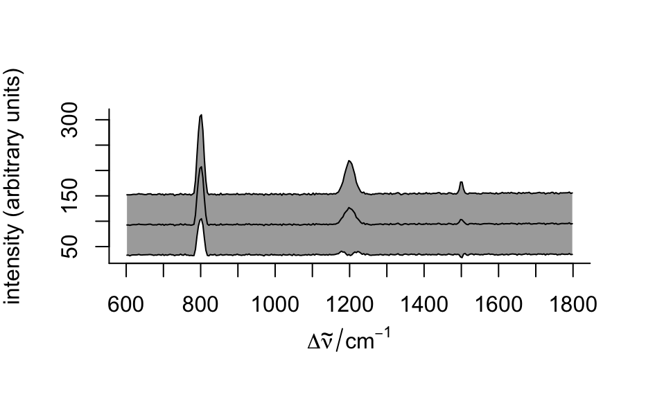
"spcprctile"

plots 16th, 50th, and 84th percentile spectra. If the distributions of the intensities at all wavelengths were normal, this would correspond to "spcmeansd". However, this is frequently not the case. Then "spcprctile" gives a better impression of the spectral data set.

"spcprctl5"

like "spcprctile", but additionally the 5th and 95th percentile spectra are plotted.

"map"

calls plotmap() to produce a map plot.

"voronoi"

calls plotvoronoi() to produce a Voronoi plot (tessellated plot, like "map" for hyperSpec objects with uneven/non-rectangular grid).

"mat"

calls plotmat() to produce a plot of the spectra matrix (not to be confused with graphics::matplot()).

"c"

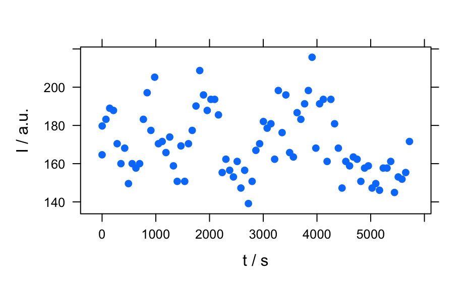
calls plotc() to produce a calibration (or time series, depth-profile, or the like).

"ts"

plots a time series: abbreviation for plotc(x, use.c = "t").

"depth"

plots a depth profile: abbreviation for plotc(x, use.c = "z").

See also

plotspc() for spectra plots (intensity over wavelength),

plotmap() for plotting maps, i.e. color coded summary value on two (usually spatial) dimensions.

plotc()

graphics::plot()

Author

C. Beleites

Examples

plot(flu)

plot(flu, "c")
#> Warning: Intensity at first wavelengh only is used.

plot(laser, "ts")
#> Warning: Intensity at first wavelengh only is used.

spc <- apply(faux_cell, 2, quantile, probs = 0.05)
spc <- sweep(faux_cell, 2, spc, "-")
plot(spc, "spcprctl5")
plot(spc, "spcprctile")
plot(spc, "spcmeansd")

### Use plotspc() as a default plot function.